Easy APA Formatted Bayesian Correlation
The Bayesian framework is the right way to go for psychological science. To facilitate its use for newcommers, we implemented the bayes_cor.test function in the psycho package, a user-friendly wrapper for the correlationBF function of the great BayesFactor package by Richard D. Morey.
Traditional Correlation
Let’s first perform a traditional correlation.
# devtools::install_github("neuropsychology/psycho.R")  # Install the latest psycho version

# Load packages
library(tidyverse)
library(psycho)

# Import data
df <- psycho::affective

cor.test(df$Concealing, df$Tolerating)
    Pearson's product-moment correlation

data:  df$Concealing and df$Tolerating
t = 2.611, df = 1249, p-value = 0.009136
alternative hypothesis: true correlation is not equal to 0
95 percent confidence interval:
 0.01832974 0.12857724
sample estimates:
       cor
0.07367859
There is a significant (whatever that means), yet weak positive correlation between Concealing and Tolerating affective styles.
Bayesian APA formatted Correlation
And now, see how quickly we can do a Bayesian correlation:
bayes_cor.test(df$Concealing, df$Tolerating)
Results of the Bayesian correlation indicate anecdotal evidence (BF = 1.95) in favour of a positive association between df$Concealing and df$Tolerating (r = 0.073, MAD = 0.028, 90% CI [0.023, 0.12]). The correlation can be considered as small or very small with respective probabilities of 16.55% and 83.06%.
The results are roughly the same, but neatly dissociate the likelihood in favour or against the null hypothesis (using the Bayes Factor), from the “significance” (wether a portion of the Credible Interval covers 0), from the effect size (interpreted here with Cohen’s (1988) rules of thumb). Critically, you can, now, simply copy/paste this output to your manuscript! It includes and formats the Bayes Factor, the median (a good point-estimate, close to the r estimated in frequentist correlation), MAD (robust equivalent of SD for median) and credible interval (CI) of the posterior distribution, as well as effect size interpretation.
Indices
We can have access to more indices with the summary:
results <- bayes_cor.test(df$Concealing, df$Tolerating)
summary(results)
| Median | MAD | Mean | SD | CI_lower | CI_higher | MPE | BF | Overlap | Rope | |
|---|---|---|---|---|---|---|---|---|---|---|
| df$Concealing/df$Tolerating | 0.07 | 0.03 | 0.07 | 0.03 | 0.03 | 0.12 | 99.56 | 1.95 | 19.43 | Undecided |
Those indices include the ROPE decision criterion (see Kruschke, 2018) as well as the Maximum Probability of Effect (MPE, the probability that an effect is negative or positive and different from 0).
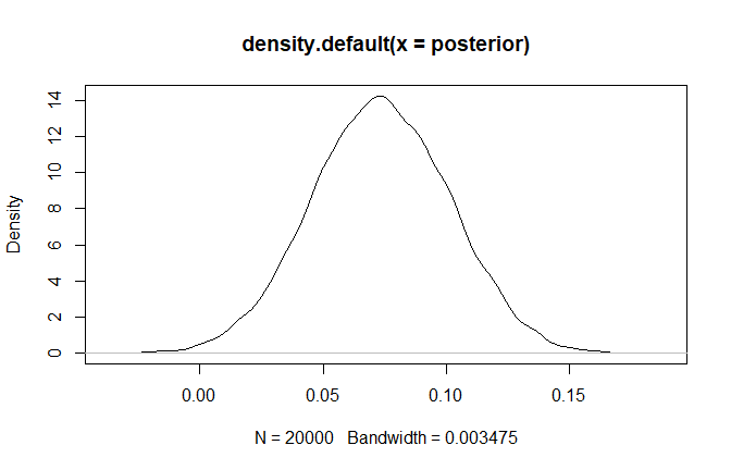
Posterior
We can easily extract the posterior distribution to visualize the probability of possible effects.
posterior <- results$values$posterior

plot(density(posterior))
Contribute
Of course, these reporting standards should change, depending on new expert recommandations or official guidelines. The goal of this package is to flexibly adaptive to new changes and good practices evolution. Therefore, if you have any advices, opinions or such, we encourage you to either let us know by opening an issue or, even better, try to implement them yourself by contributing to the code.
Credits
This package helped you? Don’t forget to cite the various packages you used :)
You can cite psycho as follows:
- Makowski, (2018). The psycho Package: an Efficient and Publishing-Oriented Workflow for Psychological Science. Journal of Open Source Software, 3(22), 470. https://doi.org/10.21105/joss.00470
Previous blogposts
- Copy/paste t-tests Directly to Manuscripts
- APA Formatted Bayesian Correlation
- Fancy Plot (with Posterior Samples) for Bayesian Regressions
- How Many Factors to Retain in Factor Analysis
- Beautiful and Powerful Correlation Tables
- Format and Interpret Linear Mixed Models
- How to do Repeated Measures ANOVAs
- Standardize (Z-score) a dataframe
- Compute Signal Detection Theory Indices