Compute Signal Detection Theory Indices with R
Signal Detection Theory Indices (dprime, beta…)
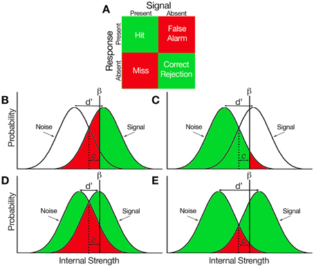
Signal detection theory (SDT) is used when psychologists want to measure the way we make decisions under conditions of uncertainty. SDT assumes that the decision maker is not a passive receiver of information, but an active decision-maker who makes difficult perceptual judgments under conditions of uncertainty. To apply signal detection theory to a data set where stimuli were either present or absent, and the observer categorized each trial as having the stimulus present or absent, the trials are sorted into one of four categories: Hit, Miss, Correct Rejection and False Alarm.

Based on the proportions of these types of trials, we can compute indices of sensitivity and response bias:
- d’ (d prime): The sensitivity. Reflects the distance between the two distributions: signal, and signal+noise and corresponds to the Z value of the hit-rate minus that of the false-alarm rate.
- beta: The bias (criterion). The value for beta is the ratio of the normal density functions at the criterion of the Z values used in the computation of d’. This reflects an observer’s bias to say ‘yes’ or ‘no’ with the unbiased observer having a value around 1.0. As the bias to say ‘yes’ increases (liberal), resulting in a higher hit-rate and false-alarm-rate, beta approaches 0.0. As the bias to say ‘no’ increases (conservative), resulting in a lower hit-rate and false-alarm rate, beta increases over 1.0 on an open-ended scale.
- A’ (aprime): Non-parametric estimate of discriminability. An A’ near 1.0 indicates good discriminability, while a value near 0.5 means chance performance.
- B’‘D (b prime prime d): Non-parametric estimate of bias. A B’‘D equal to 0.0 indicates no bias, positive numbers represent conservative bias (i.e., a tendency to answer ‘no’), negative numbers represent liberal bias (i.e. a tendency to answer ‘yes’). The maximum absolute value is 1.0.
- c: Another index of bias. the number of standard deviations from the midpoint between these two distributions, i.e., a measure on a continuum from “conservative” to “liberal”.
To compute them with psycho, simply run the following:
library(psycho)

# Let's simulate three participants with different results at a perceptual detection task
df <- data.frame(Participant = c("A", "B", "C"),
                 n_hit = c(1, 2, 5),
                 n_fa = c(1, 3, 5),
                 n_miss = c(6, 8, 1),
                 n_cr = c(4, 8, 9))

indices <- psycho::dprime(df$n_hit, df$n_fa, df$n_miss, df$n_cr)
df <- cbind(df, indices)
| Participant | n_hit | n_fa | n_miss | n_cr | dprime | beta | aprime | bppd | c |
|---|---|---|---|---|---|---|---|---|---|
| A | 1 | 1 | 6 | 4 | -0.1925836 | 0.8518485 | 0.5000000 | 0.9459459 | 0.8326077 |
| B | 2 | 3 | 8 | 8 | -0.1981923 | 0.8735807 | 0.4106061 | 0.8285714 | 0.6819377 |
| C | 5 | 5 | 1 | 9 | 0.9952151 | 0.8827453 | 0.5000000 | -0.9230769 | -0.1253182 |
Credits
This package helped you? You can cite psycho as follows:
- Makowski, (2018). The psycho Package: an Efficient and Publishing-Oriented Workflow for Psychological Science. Journal of Open Source Software, 3(22), 470. https://doi.org/10.21105/joss.00470
Previous blogposts
- Copy/paste t-tests Directly to Manuscripts
- APA Formatted Bayesian Correlation
- Fancy Plot (with Posterior Samples) for Bayesian Regressions
- How Many Factors to Retain in Factor Analysis
- Beautiful and Powerful Correlation Tables
- Format and Interpret Linear Mixed Models
- How to do Repeated Measures ANOVAs
- Standardize (Z-score) a dataframe
- Compute Signal Detection Theory Indices