Heart Rate Variability (HRV)

NeuroKit2 is the most comprehensive package when it comes to HRV indices, and this example shows how to use NeuroKit2 to compute heart rate variability (HRV) indices in the time-, frequency-, and non-linear domain.

For a comprehensive review of the most up-to-date HRV indices, a discussion of their significance in psychology, and a step-by-step guide for HRV analysis using NeuroKit2, the Heart Rate Variability in Psychology: A Review of HRV Indices and an Analysis Tutorial paper is a good place to start.

Compute HRV features

# Load the NeuroKit package
import neurokit2 as nk

Download Dataset

First, let’s download the resting rate data (sampled at 100Hz) using nk.data().

data = nk.data("bio_resting_5min_100hz")
data.head()  # Print first 5 rows

	ECG	PPG	RSP
0	0.003766	-0.102539	0.494652
1	-0.017466	-0.103760	0.502483
2	-0.015679	-0.107422	0.511102
3	-0.001598	-0.110855	0.518791
4	0.002483	-0.112610	0.528669

You can see that it consists of three different signals, pertaining to ECG, PPG (an alternative determinant of heart rate as compared to ECG), and RSP (respiration). Now, let’s extract the ECG signal in the shape of a vector (i.e., a one-dimensional array), and find the peaks using ecg_peaks().

# Find peaks
peaks, info = nk.ecg_peaks(data["ECG"], sampling_rate=100)

Note: It is critical that you specify the correct sampling rate of your signal throughout many processing functions, as this allows NeuroKit to have a time reference.

This produces two elements, peaks which is a DataFrame of same length as the input signal in which occurences of R-peaks are marked with 1 in a list of zeros. info is a dictionary of the sample points at which these R-peaks occur.

HRV is the temporal variation between consecutive heartbeats (RR intervals). Here, we will use peaks i.e. occurrences of the heartbeat peaks, as the input argument in the following HRV functions to extract the indices.

Time-Domain Analysis

First, let’s extract the time-domain indices.

# Extract clean EDA and SCR features
hrv_time = nk.hrv_time(peaks, sampling_rate=100, show=True)
hrv_time

	HRV_MeanNN	HRV_SDNN	HRV_SDANN1	HRV_SDNNI1	HRV_SDANN2	HRV_SDNNI2	HRV_SDANN5	HRV_SDNNI5	HRV_RMSSD	HRV_SDSD	...	HRV_IQRNN	HRV_SDRMSSD	HRV_Prc20NN	HRV_Prc80NN	HRV_pNN50	HRV_pNN20	HRV_MinNN	HRV_MaxNN	HRV_HTI	HRV_TINN
0	696.395349	62.135891	10.060728	60.275036	NaN	NaN	NaN	NaN	69.697983	69.779109	...	60.0	0.891502	660.0	740.0	14.651163	49.302326	470.0	1420.0	7.962963	234.375

1 rows × 25 columns

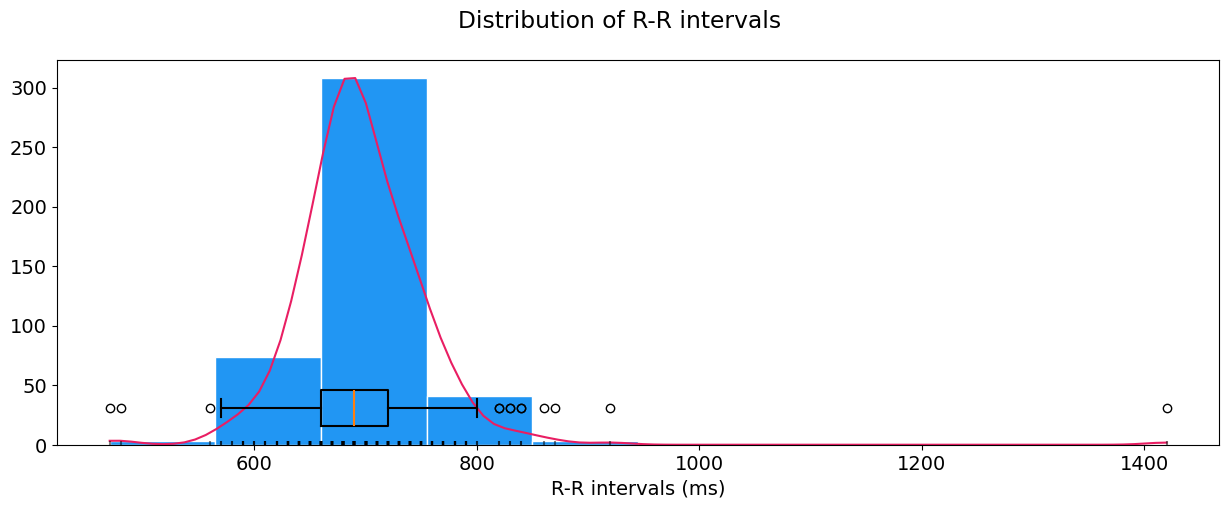
These features include the RMSSD (square root of the mean of the sum of successive differences between adjacent RR intervals), MeanNN (mean of RR intervals) so on and so forth. You can also visualize the distribution of R-R intervals by specifying show=True in hrv_time().

Frequency-Domain Analysis

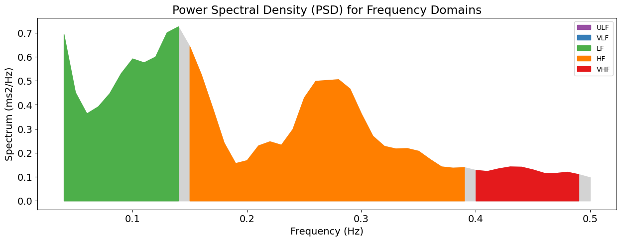
Now, let’s extract the frequency domain features, which involve extracting for example the spectral power density pertaining to different frequency bands. Again, you can visualize the power across frequency bands by specifying show=True in hrv_frequency().

hrv_freq = nk.hrv_frequency(peaks, sampling_rate=100, show=True, normalize=True)
hrv_freq

	HRV_ULF	HRV_VLF	HRV_LF	HRV_HF	HRV_VHF	HRV_TP	HRV_LFHF	HRV_LFn	HRV_HFn	HRV_LnHF
0	NaN	0.01731	0.048026	0.060232	0.011186	0.136754	0.797353	0.351186	0.44044	-2.809554

Non-Linear Domain Analysis

Now, let’s compute the non-linear indices with hrv_nonlinear().

hrv_nonlinear = nk.hrv_nonlinear(peaks, sampling_rate=100, show=True)
hrv_nonlinear

	HRV_SD1	HRV_SD2	HRV_SD1SD2	HRV_S	HRV_CSI	HRV_CVI	HRV_CSI_Modified	HRV_PIP	HRV_IALS	HRV_PSS	...	HRV_SampEn	HRV_ShanEn	HRV_FuzzyEn	HRV_MSEn	HRV_CMSEn	HRV_RCMSEn	HRV_CD	HRV_HFD	HRV_KFD	HRV_LZC
0	49.341281	72.597435	0.679656	11253.343336	1.471333	4.758252	427.259889	0.55814	0.511688	0.736041	...	1.259931	4.282683	1.063533	1.266877	1.446925	1.63037	1.209752	1.856372	1.913071	0.854475

1 rows × 56 columns

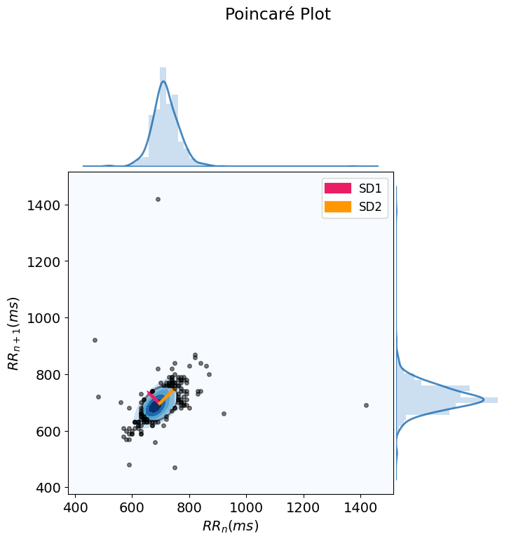
This will produce a Poincaré plot which plots each RR interval against the next successive one.

Note that there exist many more complexity indices, that are available in NeuroKit2, and that could be applied to HRV. The hrv_nonlinear() function only includes the most commonly used indices.

All Domains

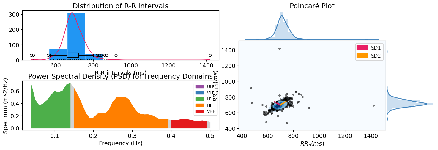
Finally, if you’d like to extract HRV indices from all three domains, you can simply input peaks into hrv(), where you can specify show=True to visualize the combination of plots depicting the RR intervals distribution, power spectral density for frequency domains, and the poincare scattergram.

hrv_indices = nk.hrv(peaks, sampling_rate=100, show=True)
hrv_indices

	HRV_MeanNN	HRV_SDNN	HRV_SDANN1	HRV_SDNNI1	HRV_SDANN2	HRV_SDNNI2	HRV_SDANN5	HRV_SDNNI5	HRV_RMSSD	HRV_SDSD	...	HRV_SampEn	HRV_ShanEn	HRV_FuzzyEn	HRV_MSEn	HRV_CMSEn	HRV_RCMSEn	HRV_CD	HRV_HFD	HRV_KFD	HRV_LZC
0	696.395349	62.135891	10.060728	60.275036	NaN	NaN	NaN	NaN	69.697983	69.779109	...	1.259931	4.282683	1.063533	1.266877	1.446925	1.63037	1.209752	1.856372	1.913071	0.854475

1 rows × 91 columns