M/EEG Microstates#

Main#

microstates_segment()#

microstates_segment(eeg, n_microstates=4, train='gfp', method='kmod', gfp_method='l1', sampling_rate=None, standardize_eeg=False, n_runs=10, max_iterations=1000, criterion='gev', random_state=None, optimize=False, **kwargs)[source]#

Segment M/EEG signal into Microstates

This functions identifies and extracts the microstates from an M/EEG signal using different clustering algorithms. Several runs of the clustering algorithm are performed, using different random initializations.The run that resulted in the best segmentation, as measured by global explained variance (GEV), is used.

kmod: Modified k-means algorithm. It differs from a traditional k-means in that it is polarity-invariant, which means that samples with EEG potential distribution maps that are similar but have opposite polarity will be assigned the same microstate class.
kmeans: Normal k-means.
kmedoids: k-medoids clustering, a more stable version of k-means.
pca: Principal Component Analysis.
ica: Independent Component Analysis.
aahc: Atomize and Agglomerate Hierarchical Clustering. Computationally heavy.

The microstates clustering is typically fitted on the EEG data at the global field power (GFP) peaks to maximize the signal to noise ratio and focus on moments of high global neuronal synchronization. It is assumed that the topography around a GFP peak remains stable and is at its highest signal-to-noise ratio at the GFP peak.

Parameters:

eeg (np.ndarray) – An array (channels, times) of M/EEG data or a Raw or Epochs object from MNE.
n_microstates (int) – The number of unique microstates to find. Defaults to 4.
train (Union[str, int, float]) – Method for selecting the timepoints how which to train the clustering algorithm. Can be "gfp" to use the peaks found in the Peaks in the global field power. Can be "all", in which case it will select all the datapoints. It can also be a number or a ratio, in which case it will select the corresponding number of evenly spread data points. For instance, train=10 will select 10 equally spaced datapoints, whereas train=0.5 will select half the data. See microstates_peaks().
method (str) – The algorithm for clustering. Can be one of "kmod" (default), "kmeans", "kmedoids", "pca", "ica", or "aahc".
gfp_method (str) – The GFP extraction method, can be either "l1" (default) or "l2" to use the L1 or L2 norm. See nk.eeg_gfp() for more details.
sampling_rate (int) – The sampling frequency of the signal (in Hz, i.e., samples/second).
standardize_eeg (bool) – Standardized (z-score) the data across time prior to GFP extraction using nk.standardize().
n_runs (int) – The number of random initializations to use for the k-means algorithm. The best fitting segmentation across all initializations is used. Defaults to 10.
max_iterations (int) – The maximum number of iterations to perform in the k-means algorithm. Defaults to 1000.
criterion (str) – Which criterion to use to choose the best run for modified k-means algorithm, can be "gev" (default) which selects the best run based on the highest global explained variance, or "cv" which selects the best run based on the lowest cross-validation criterion. See nk.microstates_gev() and nk.microstates_crossvalidation() for more details respectively.
random_state (Union[int, numpy.random.RandomState]) – The seed or RandomState for the random number generator. Defaults to None, in which case a different seed is chosen each time this function is called.
optimize (bool) – Optimized method in Poulsen et al. (2018) for the k-means modified method.

Returns:

dict – Contains information about the segmented microstates:

Microstates: The topographic maps of the found unique microstates which has a shape of n_channels x n_states
Sequence: For each sample, the index of the microstate to which the sample has been assigned.
GEV: The global explained variance of the microstates.
GFP: The global field power of the data.
Cross-Validation Criterion: The cross-validation value of the iteration.
Explained Variance: The explained variance of each cluster map generated by PCA.
Total Explained Variance: The total explained variance of the cluster maps generated by PCA.

Examples

Example 1: k-means Algorithm

In [1]: import neurokit2 as nk

# Download data
In [2]: eeg = nk.mne_data("filt-0-40_raw")

# Average rereference and band-pass filtering
In [3]: eeg = nk.eeg_rereference(eeg, 'average').filter(1, 30, verbose=False)

# Cluster microstates
In [4]: microstates = nk.microstates_segment(eeg, method="kmeans")

In [5]: nk.microstates_plot(microstates , epoch=(500, 750))

# Modified kmeans (currently comment out due to memory error)
#out_kmod = nk.microstates_segment(eeg, method='kmod')
# nk.microstates_plot(out_kmod, gfp=out_kmod["GFP"][0:500])
# K-medoids (currently comment out due to memory error)
#out_kmedoids = nk.microstates_segment(eeg, method='kmedoids')
#nk.microstates_plot(out_kmedoids, gfp=out_kmedoids["GFP"][0:500])

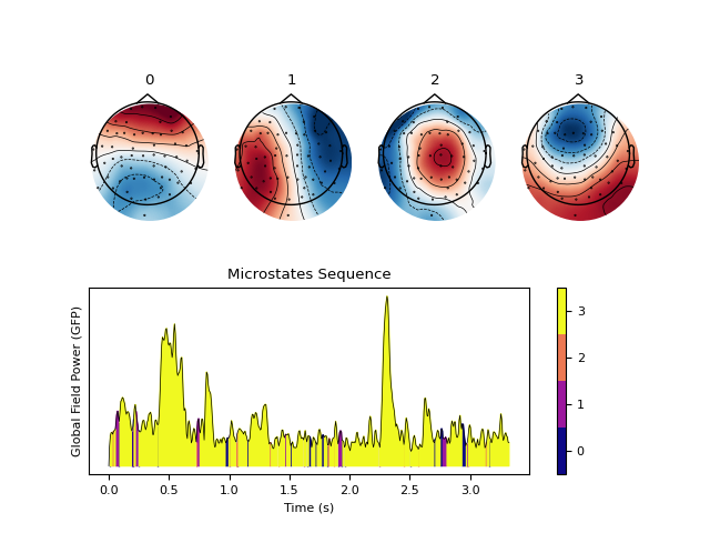
Example with PCA

In [6]: out_pca = nk.microstates_segment(eeg, method='pca', standardize_eeg=True)

In [7]: nk.microstates_plot(out_pca, gfp=out_pca["GFP"][0:500])

Example with ICA

In [8]: out_ica = nk.microstates_segment(eeg, method='ica', standardize_eeg=True)

In [9]: nk.microstates_plot(out_ica, gfp=out_ica["GFP"][0:500])

Example with AAHC

In [10]: out_aahc = nk.microstates_segment(eeg, method='aahc')

In [11]: nk.microstates_plot(out_aahc, gfp=out_aahc["GFP"][0:500])

See also

eeg_gfp, microstates_peaks, microstates_gev, microstates_crossvalidation, microstates_classify

References

Poulsen, A. T., Pedroni, A., Langer, N., & Hansen, L. K. (2018). Microstate EEGlab toolbox: an introductory guide. BioRxiv, (289850).
Pascual-Marqui, R. D., Michel, C. M., & Lehmann, D. (1995). Segmentation of brain electrical activity into microstates: model estimation and validation. IEEE Transactions on Biomedical Engineering.

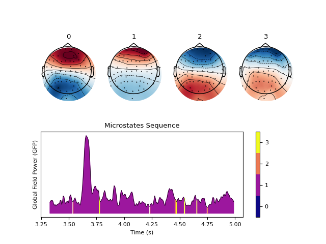
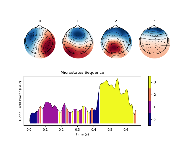
microstates_plot()#

microstates_plot(microstates, segmentation=None, gfp=None, info=None, epoch=None)[source]#

Visualize Microstates

Plots the clustered microstates.

Parameters:

microstates (np.ndarray) – The topographic maps of the found unique microstates which has a shape of n_channels x n_states, generated from microstates_segment().
segmentation (array) – For each sample, the index of the microstate to which the sample has been assigned. Defaults to None.
gfp (array) – The range of global field power (GFP) values to visualize. Defaults to None, which will plot the whole range of GFP values.
info (dict) – The dictionary output of nk.microstates_segment(). Defaults to None.
epoch (tuple) – A sub-epoch of GFP to plot in the shape (beginning sample, end sample).

Returns:

fig – Plot of prototypical microstates maps and GFP across time.

Examples

In [1]: import neurokit2 as nk

# Download data
In [2]: eeg = nk.mne_data("filt-0-40_raw")

# Average rereference and band-pass filtering
In [3]: eeg = nk.eeg_rereference(eeg, 'average').filter(1, 30, verbose=False)

# Cluster microstates
In [4]: microstates = nk.microstates_segment(eeg, method='kmeans', n_microstates=4)

In [5]: nk.microstates_plot(microstates, epoch=(500, 750))

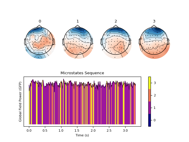
microstates_classify()#

microstates_classify(segmentation, microstates)[source]#

Reorder (sort) the microstates (experimental)

Reorder (sort) the microstates (experimental) based on the pattern of values in the vector of channels (thus, depends on how channels are ordered).

Parameters:

segmentation (Union[np.array, dict]) – Vector containing the segmentation.
microstates (Union[np.array, dict]) – Array of microstates maps . Defaults to None.

Returns:

segmentation, microstates – Tuple containing re-ordered input.

Examples

In [1]: import neurokit2 as nk

In [2]: eeg = nk.mne_data("filt-0-40_raw").filter(1, 35, verbose=False)

In [3]: eeg = nk.eeg_rereference(eeg, 'average')

# Original order
In [4]: out = nk.microstates_segment(eeg)

In [5]: nk.microstates_plot(out, gfp=out["GFP"][0:100])

# Reorder
In [6]: out = nk.microstates_classify(out["Sequence"], out["Microstates"])

microstates_clean()#

microstates_clean(eeg, sampling_rate=None, train='gfp', standardize_eeg=True, normalize=True, gfp_method='l1', **kwargs)[source]#

Prepare eeg data for microstates extraction

This is mostly a utility function to get the data ready for microstates_segment().

Parameters:

eeg (np.ndarray) – An array (channels, times) of M/EEG data or a Raw or Epochs object from MNE.
sampling_rate (int) – The sampling frequency of the signal (in Hz, i.e., samples/second). Defaults to None.
train (Union[str, int, float]) – Method for selecting the timepoints how which to train the clustering algorithm. Can be "gfp" to use the peaks found in the global field power (GFP). Can be "all", in which case it will select all the datapoints. It can also be a number or a ratio, in which case it will select the corresponding number of evenly spread data points. For instance, train=10 will select 10 equally spaced datapoints, whereas train=0.5 will select half the data. See microstates_peaks().
standardize_eeg (bool) – Standardize (z-score) the data across time using nk.standardize(), prior to GFP extraction and running k-means algorithm. Defaults to True.
normalize (bool) – Normalize (divide each data point by the maximum value of the data) across time prior to GFP extraction and running k-means algorithm. Defaults to True.
gfp_method (str) – The GFP extraction method to be passed into nk.eeg_gfp(). Can be either "l1" (default) or "l2" to use the L1 or L2 norm.
**kwargs (optional) – Other arguments.

Returns:

eeg (array) – The eeg data which has a shape of channels x samples.
peaks (array) – The index of the sample where GFP peaks occur.
gfp (array) – The global field power of each sample point in the data.
info (dict) – Other information pertaining to the eeg raw object.

Examples

In [1]: import neurokit2 as nk

In [2]: eeg = nk.mne_data("filt-0-40_raw")

In [3]: eeg, peaks, gfp, info = nk.microstates_clean(eeg, train="gfp")

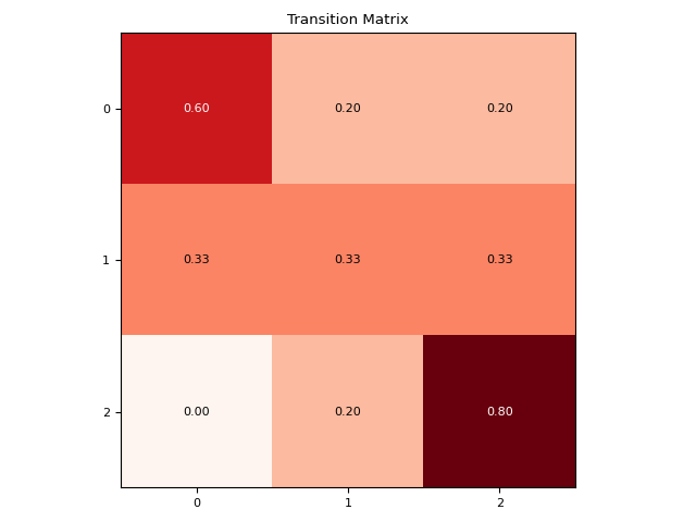
microstates_dynamic()#

microstates_dynamic(microstates, show=False)[source]#

Dynamic Properties of Microstates

This computes statistics related to the transition pattern (based on the transition_matrix()).

Note

This function does not compute all the features available under the markov submodule. Don’t hesitate to open an issue to help us test and decide what features to include.

Parameters:

microstates (np.ndarray) – The topographic maps of the found unique microstates which has a shape of n_channels x n_states, generated from nk.microstates_segment().
show (bool) – Show the transition matrix.

Returns:

DataFrame – Dynamic properties of microstates.

Examples

In [1]: import neurokit2 as nk

In [2]: microstates = [0, 0, 0, 1, 1, 2, 2, 2, 2, 1, 0, 0, 2, 2]

In [3]: nk.microstates_dynamic(microstates, show=True)
Out[3]: 
   Microstate_0_to_0  Microstate_0_to_1  ...  Microstate_2_to_1  Microstate_2_to_2
0                0.6                0.2  ...                0.2                0.8

[1 rows x 9 columns]

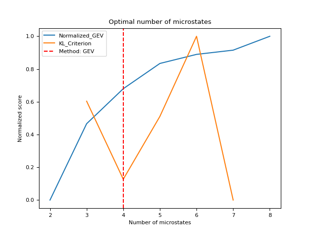
microstates_findnumber()#

microstates_findnumber(eeg, n_max=12, method='GEV', clustering_method='kmod', show=False, verbose=True, **kwargs)[source]#

Estimate optimal number of microstates

Computes statistical indices useful for estimating the optimal number of microstates using a

Global Explained Variance (GEV): measures how similar each EEG sample is to its assigned microstate class. The higher (closer to 1), the better the segmentation.
Krzanowski-Lai Criterion (KL): measures quality of microstate segmentation based on the dispersion measure (average distance between samples in the same microstate class); the larger the KL value, the better the segmentation. Note that KL is not a polarity invariant measure and thus might not be a suitable measure of fit for polarity-invariant methods such as modified K-means and (T)AAHC.

Parameters:

eeg (np.ndarray) – An array (channels, times) of M/EEG data or a Raw or Epochs object from MNE.
n_max (int) – Maximum number of microstates to try. A higher number leads to a longer process.
method (str) – The method to use to estimate the optimal number of microstates. Can be “GEV” (the elbow, detected using find_knee()), or “KL” (the location of the maximum value).
show (bool) – Plot indices normalized on the same scale.
verbose (bool) – Print progress bar.
**kwargs – Arguments to be passed to microstates_segment()

Returns:

int – Optimal number of microstates.
DataFrame – The different quality scores for each number of microstates.

See also

microstates_segment

Examples

In [1]: import neurokit2 as nk

In [2]: eeg = nk.mne_data("filt-0-40_raw").crop(0, 5)

# Estimate optimal number
In [3]: n_clusters, results = nk.microstates_findnumber(eeg, n_max=8, show=True)
[........................................] 0/7
[█████...................................] 1/7
[███████████.............................] 2/7
[█████████████████.......................] 3/7
[██████████████████████..................] 4/7
[████████████████████████████............] 5/7
[██████████████████████████████████......] 6/7
[████████████████████████████████████████] 7/7

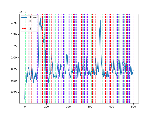
microstates_peaks()#

microstates_peaks(eeg, gfp=None, sampling_rate=None, distance_between=0.01, **kwargs)[source]#

Find peaks of stability using the GFP

Peaks in the global field power (GFP) are often used to find microstates.

Parameters:

eeg (np.ndarray) – An array (channels, times) of M/EEG data or a Raw or Epochs object from MNE.
gfp (list) – The Global Field Power (GFP). If None, will be obtained via eeg_gfp().
sampling_rate (int) – The sampling frequency of the signal (in Hz, i.e., samples/second).
distance_between (float) – The minimum distance (this value is to be multiplied by the sampling rate) between peaks. The default is 0.01, which corresponds to 10 ms (as suggested in the Microstate EEGlab toolbox).
**kwargs – Additional arguments to be passed to eeg_gfp().

Returns:

peaks (array) – The index of the sample where GFP peaks occur.

Examples

In [1]: import neurokit2 as nk

In [2]: eeg = nk.mne_data("filt-0-40_raw")

In [3]: gfp = nk.eeg_gfp(eeg)

In [4]: peaks1 = nk.microstates_peaks(eeg, distance_between=0.01)

In [5]: peaks2 = nk.microstates_peaks(eeg, distance_between=0.05)

In [6]: peaks3 = nk.microstates_peaks(eeg, distance_between=0.10)

In [7]: nk.events_plot([peaks1[peaks1 < 500], peaks2[peaks2 < 500], peaks3[peaks3 < 500]], gfp[0:500])

See also

eeg_gfp

microstates_static()#

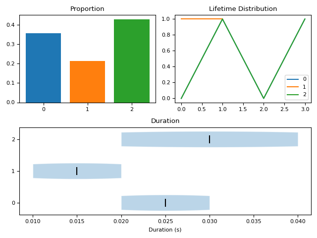
microstates_static(microstates, sampling_rate=1000, show=False)[source]#

Static Properties of Microstates

The duration of each microstate is also referred to as the Ratio of Time Covered (RTT) in some microstates publications.

Parameters:

microstates (np.ndarray) – The sequence .
sampling_rate (int) – The sampling frequency of the signal (in Hz, i.e., samples/second). Defaults to 1000.
show (bool) – Returns a plot of microstate duration, proportion, and lifetime distribution if True.

Returns:

DataFrame – Values of microstates proportion, lifetime distribution and duration (median, mean, and their averages).

See also

microstates_dynamic

Examples

In [1]: import neurokit2 as nk

In [2]: microstates = [0, 0, 0, 1, 1, 2, 2, 2, 2, 1, 0, 0, 2, 2]

In [3]: nk.microstates_static(microstates, sampling_rate=100, show=True)
Out[3]: 
   Microstate_0_Proportion  ...  Microstate_Average_DurationMedian
0                 0.357143  ...                               0.02

[1 rows x 14 columns]

M/EEG Microstates

Contents

M/EEG Microstates#

Main#

microstates_segment()#

microstates_plot()#

microstates_classify()#

microstates_clean()#

microstates_dynamic()#

microstates_findnumber()#

microstates_peaks()#

microstates_static()#