Signal Processing

Signal Processing#

Preprocessing#

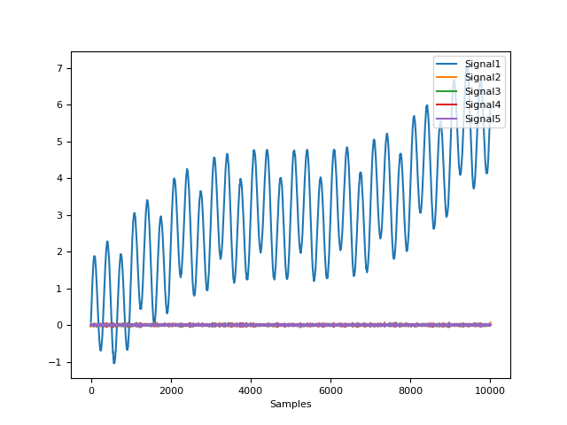
signal_simulate()#

signal_simulate(duration=10, sampling_rate=1000, frequency=1, amplitude=0.5, noise=0, silent=False, random_state=None)[source]#

Simulate a continuous signal

Parameters:

duration (float) – Desired length of duration (s).
sampling_rate (int) – The desired sampling rate (in Hz, i.e., samples/second).
frequency (float or list) – Oscillatory frequency of the signal (in Hz, i.e., oscillations per second).
amplitude (float or list) – Amplitude of the oscillations.
noise (float) – Noise level (amplitude of the laplace noise).
silent (bool) – If False (default), might print warnings if impossible frequencies are queried.
random_state (None, int, numpy.random.RandomState or numpy.random.Generator) – Seed for the random number generator. See for misc.check_random_state for further information.

Returns:

array – The simulated signal.

Examples

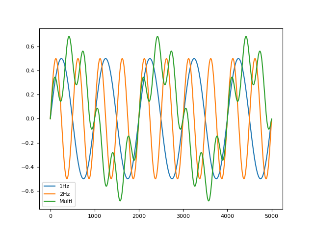
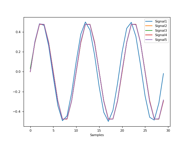
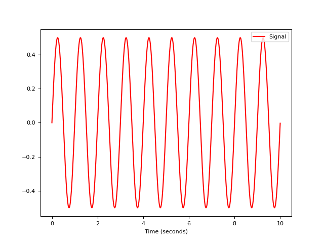
In [1]: import pandas as pd

In [2]: import neurokit2 as nk

In [3]: pd.DataFrame({
   ...:     "1Hz": nk.signal_simulate(duration=5, frequency=1),
   ...:     "2Hz": nk.signal_simulate(duration=5, frequency=2),
   ...:     "Multi": nk.signal_simulate(duration=5, frequency=[0.5, 3], amplitude=[0.5, 0.2])
   ...: }).plot()
   ...: 
Out[3]: <Axes: >

signal_filter()#

signal_filter(signal, sampling_rate=1000, lowcut=None, highcut=None, method='butterworth', order=2, window_size='default', powerline=50, show=False)[source]#

Signal filtering

Filter a signal using different methods such as “butterworth”, “fir”, “savgol” or “powerline” filters.

Apply a lowpass (if “highcut” frequency is provided), highpass (if “lowcut” frequency is provided) or bandpass (if both are provided) filter to the signal.

Parameters:

signal (Union[list, np.array, pd.Series]) – The signal (i.e., a time series) in the form of a vector of values.
sampling_rate (int) – The sampling frequency of the signal (in Hz, i.e., samples/second).
lowcut (float) – Lower cutoff frequency in Hz. The default is None.
highcut (float) – Upper cutoff frequency in Hz. The default is None.
method (str) – Can be one of "butterworth", "fir", "bessel" or "savgol". Note that for Butterworth, the function uses the SOS method from scipy.signal.sosfiltfilt(), recommended for general purpose filtering. One can also specify "butterworth_ba" for a more traditional and legacy method (often implemented in other software).
order (int) – Only used if method is "butterworth" or "savgol". Order of the filter (default is 2).
window_size (int) – Only used if method is "savgol". The length of the filter window (i.e. the number of coefficients). Must be an odd integer. If default, will be set to the sampling rate divided by 10 (101 if the sampling rate is 1000 Hz).
powerline (int) – Only used if method is "powerline". The powerline frequency (normally 50 Hz or 60Hz).
show (bool) – If True, plot the filtered signal as an overlay of the original.

See also

signal_detrend, signal_psd

Returns:: array – Vector containing the filtered signal.

Examples

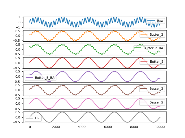
In [1]: import numpy as np

In [2]: import pandas as pd

In [3]: import neurokit2 as nk

In [4]: signal = nk.signal_simulate(duration=10, frequency=0.5) # Low freq

In [5]: signal += nk.signal_simulate(duration=10, frequency=5) # High freq

# Visualize Lowpass Filtered Signal using Different Methods
In [6]: fig1 = pd.DataFrame({"Raw": signal,
   ...:                    "Butter_2": nk.signal_filter(signal, highcut=3, method="butterworth",
   ...:                     order=2),
   ...:                    "Butter_2_BA": nk.signal_filter(signal, highcut=3,
   ...:                     method="butterworth_ba", order=2),
   ...:                    "Butter_5": nk.signal_filter(signal, highcut=3, method="butterworth",
   ...:                     order=5),
   ...:                    "Butter_5_BA": nk.signal_filter(signal, highcut=3,
   ...:                     method="butterworth_ba", order=5),
   ...:                    "Bessel_2": nk.signal_filter(signal, highcut=3, method="bessel", order=2),
   ...:                    "Bessel_5": nk.signal_filter(signal, highcut=3, method="bessel", order=5),
   ...:                    "FIR": nk.signal_filter(signal, highcut=3, method="fir")}).plot(subplots=True)
   ...: 

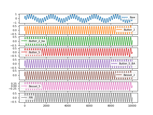
# Visualize Highpass Filtered Signal using Different Methods
In [7]: fig2 = pd.DataFrame({"Raw": signal,
   ...:                     "Butter_2": nk.signal_filter(signal, lowcut=2, method="butterworth",
   ...:                     order=2),
   ...:                     "Butter_2_ba": nk.signal_filter(signal, lowcut=2,
   ...:                     method="butterworth_ba", order=2),
   ...:                     "Butter_5": nk.signal_filter(signal, lowcut=2, method="butterworth",
   ...:                     order=5),
   ...:                     "Butter_5_BA": nk.signal_filter(signal, lowcut=2,
   ...:                     method="butterworth_ba", order=5),
   ...:                     "Bessel_2": nk.signal_filter(signal, lowcut=2, method="bessel", order=2),
   ...:                     "Bessel_5": nk.signal_filter(signal, lowcut=2, method="bessel", order=5),
   ...:                     "FIR": nk.signal_filter(signal, lowcut=2, method="fir")}).plot(subplots=True)
   ...: 

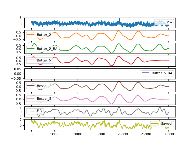
# Using Bandpass Filtering in real-life scenarios
# Simulate noisy respiratory signal
In [8]: original = nk.rsp_simulate(duration=30, method="breathmetrics", noise=0)

In [9]: signal = nk.signal_distort(original, noise_frequency=[0.1, 2, 10, 100], noise_amplitude=1,
   ...:                           powerline_amplitude=1)
   ...: 

# Bandpass between 10 and 30 breaths per minute (respiratory rate range)
In [10]: fig3 = pd.DataFrame({"Raw": signal,
   ....:                      "Butter_2": nk.signal_filter(signal, lowcut=10/60, highcut=30/60,
   ....:                                                   method="butterworth", order=2),
   ....:                      "Butter_2_BA": nk.signal_filter(signal, lowcut=10/60, highcut=30/60,
   ....:                                                      method="butterworth_ba", order=2),
   ....:                      "Butter_5": nk.signal_filter(signal, lowcut=10/60, highcut=30/60,
   ....:                                                   method="butterworth", order=5),
   ....:                      "Butter_5_BA": nk.signal_filter(signal, lowcut=10/60, highcut=30/60,
   ....:                                                      method="butterworth_ba", order=5),
   ....:                      "Bessel_2": nk.signal_filter(signal, lowcut=10/60, highcut=30/60,
   ....:                                                   method="bessel", order=2),
   ....:                      "Bessel_5": nk.signal_filter(signal, lowcut=10/60, highcut=30/60,
   ....:                                                   method="bessel", order=5),
   ....:                      "FIR": nk.signal_filter(signal, lowcut=10/60, highcut=30/60,
   ....:                                              method="fir"),
   ....:                      "Savgol": nk.signal_filter(signal, method="savgol")}).plot(subplots=True)
   ....: 

signal_sanitize()#

signal_sanitize(signal)[source]#

Signal input sanitization

Reset indexing for Pandas Series.

Parameters:: signal (Series) – The indexed input signal (pandas Dataframe.set_index())
Returns:: Series – The default indexed signal

Examples

In [1]: import pandas as pd

In [2]: import neurokit2 as nk

In [3]: signal = nk.signal_simulate(duration=10, sampling_rate=1000, frequency=1)

In [4]: df = pd.DataFrame({'signal': signal, 'id': [x*2 for x in range(len(signal))]})

In [5]: df = df.set_index('id')

In [6]: default_index_signal = nk.signal_sanitize(df.signal)

signal_resample()#

signal_resample(signal, desired_length=None, sampling_rate=None, desired_sampling_rate=None, method='interpolation')[source]#

Resample a continuous signal to a different length or sampling rate

Up- or down-sample a signal. The user can specify either a desired length for the vector, or input the original sampling rate and the desired sampling rate.

Parameters:

signal (Union[list, np.array, pd.Series]) – The signal (i.e., a time series) in the form of a vector of values.
desired_length (int) – The desired length of the signal.
sampling_rate (int) – The original sampling frequency (in Hz, i.e., samples/second).
desired_sampling_rate (int) – The desired (output) sampling frequency (in Hz, i.e., samples/second).
method (str) – Can be "interpolation" (see scipy.ndimage.zoom()), "numpy" for numpy’s interpolation (see np.interp()),``”pandas”`` for Pandas’ time series resampling, "poly" (see scipy.signal.resample_poly()) or "FFT" (see scipy.signal.resample()) for the Fourier method. "FFT" is the most accurate (if the signal is periodic), but becomes exponentially slower as the signal length increases. In contrast, "interpolation" is the fastest, followed by "numpy", "poly" and "pandas".

Returns:

array – Vector containing resampled signal values.

See also

signal_interpolate

Examples

Example 1: Downsampling

In [1]: import numpy as np

In [2]: import pandas as pd

In [3]: import neurokit2 as nk

In [4]: signal = nk.signal_simulate(duration=1, sampling_rate=500, frequency=3)

# Downsample
In [5]: data = {}

In [6]: for m in ["interpolation", "FFT", "poly", "numpy", "pandas"]:
   ...:     data[m] = nk.signal_resample(signal, sampling_rate=500, desired_sampling_rate=30, method=m)
   ...: 

In [7]: nk.signal_plot([data[m] for m in data.keys()])

Example 2: Upsampling

In [8]: signal = nk.signal_simulate(duration=1, sampling_rate=30, frequency=3)

# Upsample
In [9]: data = {}

In [10]: for m in ["interpolation", "FFT", "poly", "numpy", "pandas"]:
   ....:     data[m] = nk.signal_resample(signal, sampling_rate=30, desired_sampling_rate=500, method=m)
   ....: 

In [11]: nk.signal_plot([data[m] for m in data.keys()], labels=list(data.keys()))

Example 3: Benchmark

In [13]: signal = nk.signal_simulate(duration=1, sampling_rate=1000, frequency=3)

# Timing benchmarks
In [14]: %timeit nk.signal_resample(signal, method="interpolation",
   ....:                            sampling_rate=1000, desired_sampling_rate=500)
   ....: %timeit nk.signal_resample(signal, method="FFT",
   ....:                            sampling_rate=1000, desired_sampling_rate=500)
   ....: %timeit nk.signal_resample(signal, method="poly",
   ....:                            sampling_rate=1000, desired_sampling_rate=500)
   ....: %timeit nk.signal_resample(signal, method="numpy",
   ....:                            sampling_rate=1000, desired_sampling_rate=500)
   ....: %timeit nk.signal_resample(signal, method="pandas",
   ....:                            sampling_rate=1000, desired_sampling_rate=500)
   ....: 

signal_fillmissing()#

signal_fillmissing(signal, method='both')[source]#

Handle missing values

Fill missing values in a signal using specific methods.

Parameters:

signal (Union[list, np.array, pd.Series]) – The signal (i.e., a time series) in the form of a vector of values.
method (str) – The method to use to fill missing values. Can be one of "forward", "backward", or "both". The default is "both".

Returns:

signal

Examples

In [1]: import neurokit2 as nk

In [2]: signal = [np.nan, 1, 2, 3, np.nan, np.nan, 6, 7, np.nan]

In [3]: nk.signal_fillmissing(signal, method="forward")
Out[3]: array([nan,  1.,  2.,  3.,  3.,  3.,  6.,  7.,  7.])

In [4]: nk.signal_fillmissing(signal, method="backward")
Out[4]: array([ 1.,  1.,  2.,  3.,  6.,  6.,  6.,  7., nan])

In [5]: nk.signal_fillmissing(signal, method="both")
Out[5]: array([1., 1., 2., 3., 3., 3., 6., 7., 7.])

Transformation#

signal_binarize()#

signal_binarize(signal, method='threshold', threshold='auto')[source]#

Binarize a continuous signal

Convert a continuous signal into zeros and ones depending on a given threshold.

Parameters:

signal (Union[list, np.array, pd.Series]) – The signal (i.e., a time series) in the form of a vector of values.
method (str) – The algorithm used to discriminate between the two states. Can be one of "mixture" (default) or "threshold". If "mixture", will use a Gaussian Mixture Model to categorize between the two states. If "threshold", will consider as activated all points which value is superior to the threshold.
threshold (float) – If method is "mixture", then it corresponds to the minimum probability required to be considered as activated (if "auto", then 0.5). If method is "threshold", then it corresponds to the minimum amplitude to detect as onset. If "auto", takes the value between the max and the min.

Returns:

list – A list or array depending on the type passed.

Examples

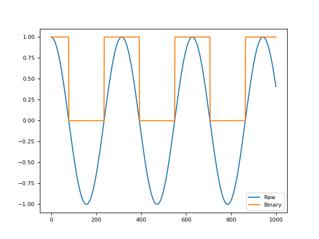
In [1]: import neurokit2 as nk

In [2]: import numpy as np

In [3]: import pandas as pd

In [4]: signal = np.cos(np.linspace(start=0, stop=20, num=1000))

In [5]: binary = nk.signal_binarize(signal)

In [6]: pd.DataFrame({"Raw": signal, "Binary": binary}).plot()
Out[6]: <Axes: >

signal_decompose()#

signal_decompose(signal, method='emd', n_components=None, **kwargs)[source]#

Decompose a signal

Signal decomposition into different sources using different methods, such as Empirical Mode Decomposition (EMD) or Singular spectrum analysis (SSA)-based signal separation method.

The extracted components can then be recombined into meaningful sources using signal_recompose().

Parameters:

signal (Union[list, np.array, pd.Series]) – Vector of values.
method (str) – The decomposition method. Can be one of "emd" or "ssa".
n_components (int) – Number of components to extract. Only used for "ssa" method. If None, will default to 50.
**kwargs – Other arguments passed to other functions.

Returns:

Array – Components of the decomposed signal.

See also

signal_recompose

Examples

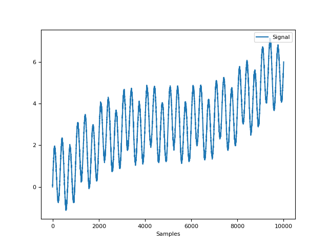
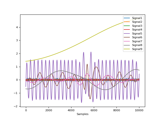
In [1]: import neurokit2 as nk

# Create complex signal
In [2]: signal = nk.signal_simulate(duration=10, frequency=1, noise=0.01)  # High freq

In [3]: signal += 3 * nk.signal_simulate(duration=10, frequency=3, noise=0.01)  # Higher freq

In [4]: signal += 3 * np.linspace(0, 2, len(signal))  # Add baseline and trend

In [5]: signal += 2 * nk.signal_simulate(duration=10, frequency=0.1, noise=0)

In [6]: nk.signal_plot(signal)

# Example 1: Using the EMD method
In [7]: components = nk.signal_decompose(signal, method="emd")

# Visualize Decomposed Signal Components
In [8]: nk.signal_plot(components)

# Example 2: USing the SSA method
In [9]: components = nk.signal_decompose(signal, method="ssa", n_components=5)

# Visualize Decomposed Signal Components
In [10]: nk.signal_plot(components)  # Visualize components

signal_recompose()#

signal_recompose(components, method='wcorr', threshold=0.5, keep_sd=None, **kwargs)[source]#

Combine signal sources after decomposition

Combine and reconstruct meaningful signal sources after signal decomposition.

Parameters:

components (array) – Array of components obtained via signal_decompose().
method (str) – The decomposition method. Can be one of "wcorr".
threshold (float) – The threshold used to group components together.
keep_sd (float) – If a float is specified, will only keep the reconstructed components that are superior or equal to that percentage of the max standard deviaiton (SD) of the components. For instance, keep_sd=0.01 will remove all components with SD lower than 1% of the max SD. This can be used to filter out noise.
**kwargs – Other arguments used to override, for instance metric="chebyshev".

Returns:

Array – Components of the recomposed components.

Examples

In [1]: import neurokit2 as nk

# Create complex signal
In [2]: signal = nk.signal_simulate(duration=10, frequency=1, noise=0.01)  # High freq

In [3]: signal += 3 * nk.signal_simulate(duration=10, frequency=3, noise=0.01)  # Higher freq

In [4]: signal += 3 * np.linspace(0, 2, len(signal))  # Add baseline and trend

In [5]: signal += 2 * nk.signal_simulate(duration=10, frequency=0.1, noise=0)

# Decompose signal
In [6]: components = nk.signal_decompose(signal, method='emd')

# Recompose
In [7]: recomposed = nk.signal_recompose(components, method='wcorr', threshold=0.90)

In [8]: nk.signal_plot(components)  # Visualize components

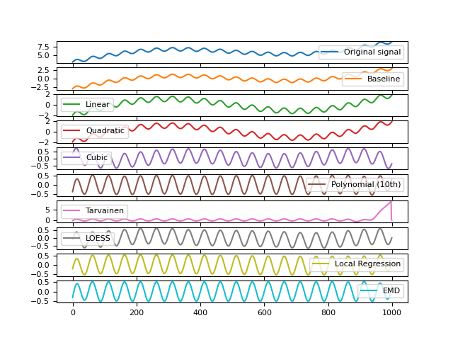
signal_detrend()#

signal_detrend(signal, method='polynomial', order=1, regularization=500, alpha=0.75, window=1.5, stepsize=0.02, components=[-1], sampling_rate=1000)[source]#

Signal Detrending Apply a baseline (order = 0), linear (order = 1), or polynomial (order > 1) detrending to the signal (i.e., removing a general trend). One can also use other methods, such as smoothness priors approach described by Tarvainen (2002) or LOESS regression, but these scale badly for long signals. :Parameters: * signal (Union[list, np.array, pd.Series]) – The signal (i.e., a time series) in the form of a vector of values.

method (str) – Can be one of "polynomial" (default; traditional detrending of a given order) or "tarvainen2002" to use the smoothness priors approach described by Tarvainen (2002) (mostly used in HRV analyses as a lowpass filter to remove complex trends), "loess" for LOESS smoothing trend removal or "locreg" for local linear regression (the ‘runline’ algorithm from chronux).

order (int) – Only used if method is "polynomial". The order of the polynomial. 0, 1 or > 1 for a baseline (‘constant detrend’, i.e., remove only the mean), linear (remove the linear trend) or polynomial detrending, respectively. Can also be "auto", in which case it will attempt to find the optimal order to minimize the RMSE.

regularization (int) – Only used if method="tarvainen2002". The regularization parameter (default to 500).

alpha (float) – Only used if method is “loess”. The parameter which controls the degree of smoothing.

window (float) – Only used if method is “locreg”. The detrending window should correspond to the 1 divided by the desired low-frequency band to remove (window = 1 / detrend_frequency) For instance, to remove frequencies below 0.67Hz the window should be 1.5 (1 / 0.67 = 1.5).

stepsize (float) – Only used if method is "locreg".

components (list) – Only used if method is "EMD". What Intrinsic Mode Functions (IMFs) from EMD to remove. By default, the last one.

sampling_rate (int, optional) – Only used if method is “locreg”. Sampling rate (Hz) of the signal. If not None, the stepsize and window arguments will be multiplied by the sampling rate. By default 1000.

Returns:: array – Vector containing the detrended signal.

Examples

In [1]: import numpy as np

In [2]: import pandas as pd

In [3]: import neurokit2 as nk

In [4]: import matplotlib.pyplot as plt

# Simulate signal with low and high frequency
In [5]: signal = nk.signal_simulate(frequency=[0.1, 2], amplitude=[2, 0.5], sampling_rate=100)

In [6]: signal = signal + (3 + np.linspace(0, 6, num=len(signal)))  # Add baseline and linear trend

# Apply detrending algorithms
# ---------------------------
# Method 1: Default Polynomial Detrending of a Given Order
# Constant detrend (removes the mean)
In [7]: baseline = nk.signal_detrend(signal, order=0)

# Linear Detrend (removes the linear trend)
In [8]: linear = nk.signal_detrend(signal, order=1)

# Polynomial Detrend (removes the polynomial trend)
In [9]: quadratic = nk.signal_detrend(signal, order=2)  # Quadratic detrend

In [10]: cubic = nk.signal_detrend(signal, order=3)  # Cubic detrend

In [11]: poly10 = nk.signal_detrend(signal, order=10)  # Linear detrend (10th order)

# Method 2: Tarvainen's smoothness priors approach (Tarvainen et al., 2002)
In [12]: tarvainen = nk.signal_detrend(signal, method="tarvainen2002")

# Method 3: LOESS smoothing trend removal
In [13]: loess = nk.signal_detrend(signal, method="loess")

# Method 4: Local linear regression (100Hz)
In [14]: locreg = nk.signal_detrend(signal, method="locreg",
   ....:                            window=1.5, stepsize=0.02, sampling_rate=100)
   ....: 

# Method 5: EMD
In [15]: emd = nk.signal_detrend(signal, method="EMD", components=[-2, -1])

# Visualize different methods
In [16]: axes = pd.DataFrame({"Original signal": signal,
   ....:                     "Baseline": baseline,
   ....:                     "Linear": linear,
   ....:                     "Quadratic": quadratic,
   ....:                     "Cubic": cubic,
   ....:                     "Polynomial (10th)": poly10,
   ....:                     "Tarvainen": tarvainen,
   ....:                     "LOESS": loess,
   ....:                     "Local Regression": locreg,
   ....:                     "EMD": emd}).plot(subplots=True)
   ....: 

# Plot horizontal lines to better visualize the detrending
In [17]: for subplot in axes:
   ....:     subplot.axhline(y=0, color="k", linestyle="--")
   ....: 

References

Tarvainen, M. P., Ranta-Aho, P. O., & Karjalainen, P. A. (2002). An advanced detrending method with application to HRV analysis. IEEE Transactions on Biomedical Engineering, 49(2), 172-175

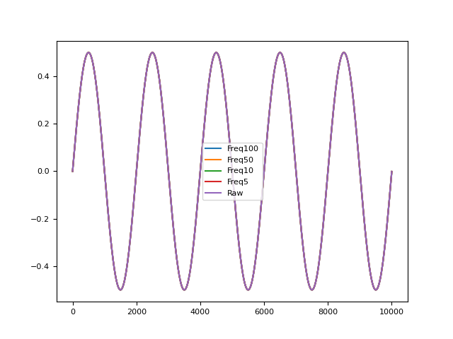
signal_distort()#

signal_distort(signal, sampling_rate=1000, noise_shape='laplace', noise_amplitude=0, noise_frequency=100, powerline_amplitude=0, powerline_frequency=50, artifacts_amplitude=0, artifacts_frequency=100, artifacts_number=5, linear_drift=False, random_state=None, silent=False)[source]#

Signal distortion

Add noise of a given frequency, amplitude and shape to a signal.

Parameters:

signal (Union[list, np.array, pd.Series]) – The signal (i.e., a time series) in the form of a vector of values.
sampling_rate (int) – The sampling frequency of the signal (in Hz, i.e., samples/second).
noise_shape (str) – The shape of the noise. Can be one of "laplace" (default) or "gaussian".
noise_amplitude (float) – The amplitude of the noise (the scale of the random function, relative to the standard deviation of the signal).
noise_frequency (float) – The frequency of the noise (in Hz, i.e., samples/second).
powerline_amplitude (float) – The amplitude of the powerline noise (relative to the standard deviation of the signal).
powerline_frequency (float) – The frequency of the powerline noise (in Hz, i.e., samples/second).
artifacts_amplitude (float) – The amplitude of the artifacts (relative to the standard deviation of the signal).
artifacts_frequency (int) – The frequency of the artifacts (in Hz, i.e., samples/second).
artifacts_number (int) – The number of artifact bursts. The bursts have a random duration between 1 and 10% of the signal duration.
linear_drift (bool) – Whether or not to add linear drift to the signal.
random_state (None, int, numpy.random.RandomState or numpy.random.Generator) – Seed for the random number generator. See for misc.check_random_state for further information.
silent (bool) – Whether or not to display warning messages.

Returns:

array – Vector containing the distorted signal.

Examples

In [1]: import numpy as np

In [2]: import pandas as pd

In [3]: import neurokit2 as nk

In [4]: signal = nk.signal_simulate(duration=10, frequency=0.5)

# Noise
In [5]: noise = pd.DataFrame({"Freq100": nk.signal_distort(signal, noise_frequency=200),
   ...:                      "Freq50": nk.signal_distort(signal, noise_frequency=50),
   ...:                      "Freq10": nk.signal_distort(signal, noise_frequency=10),
   ...:                      "Freq5": nk.signal_distort(signal, noise_frequency=5),
   ...:                      "Raw": signal}).plot()
   ...: 

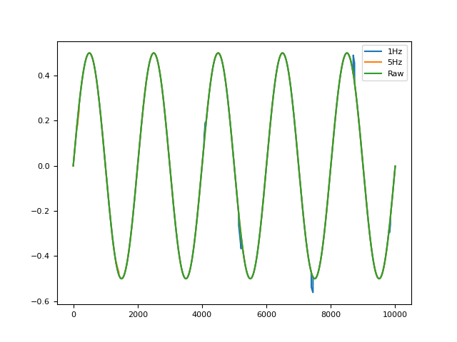
# Artifacts
In [6]: artifacts = pd.DataFrame({"1Hz": nk.signal_distort(signal, noise_amplitude=0,
   ...:                                                   artifacts_frequency=1,
   ...:                                                   artifacts_amplitude=0.5),
   ...:                          "5Hz": nk.signal_distort(signal, noise_amplitude=0,
   ...:                                                   artifacts_frequency=5,
   ...:                                                   artifacts_amplitude=0.2),
   ...:                          "Raw": signal}).plot()
   ...: 

signal_flatline()#

signal_flatline(signal, threshold=0.01)[source]#

Return the Flatline Percentage of the Signal

Parameters:

signal (Union[list, np.array, pd.Series]) – The signal (i.e., a time series) in the form of a vector of values.
threshold (float, optional) – Flatline threshold relative to the biggest change in the signal. This is the percentage of the maximum value of absolute consecutive differences.

Returns:

float – Percentage of signal where the absolute value of the derivative is lower then the threshold.

Examples

In [1]: import neurokit2 as nk

In [2]: signal = nk.signal_simulate(duration=5)

In [3]: nk.signal_flatline(signal)
Out[3]: 0.008

signal_interpolate()#

signal_interpolate(x_values, y_values=None, x_new=None, method='quadratic', fill_value=None)[source]#

Interpolate a signal

Interpolate a signal using different methods.

Parameters:

x_values (Union[list, np.array, pd.Series]) – The samples corresponding to the values to be interpolated.
y_values (Union[list, np.array, pd.Series]) – The values to be interpolated. If not provided, any NaNs in the x_values will be interpolated with _signal_interpolate_nan(), considering the x_values as equally spaced.
x_new (Union[list, np.array, pd.Series] or int) – The samples at which to interpolate the y_values. Samples before the first value in x_values or after the last value in x_values will be extrapolated. If an integer is passed, nex_x will be considered as the desired length of the interpolated signal between the first and the last values of x_values. No extrapolation will be done for values before or after the first and the last values of x_values.
method (str) – Method of interpolation. Can be "linear", "nearest", "zero", "slinear", "quadratic", "cubic", "previous", "next", "monotone_cubic", or "akima". The methods "zero", "slinear",``”quadratic”`` and "cubic" refer to a spline interpolation of zeroth, first, second or third order; whereas "previous" and "next" simply return the previous or next value of the point. An integer specifying the order of the spline interpolator to use. See here for details on the "monotone_cubic" method. See here for details on the "akima" method.
fill_value (float or tuple or str) – If a ndarray (or float), this value will be used to fill in for requested points outside of the data range. If a two-element tuple, then the first element is used as a fill value for x_new < x[0] and the second element is used for x_new > x[-1]. If “extrapolate”, then points outside the data range will be extrapolated. If not provided, then the default is ([y_values[0]], [y_values[-1]]).

Returns:

array – Vector of interpolated samples.

See also

signal_resample

Examples

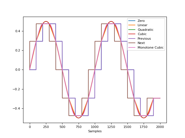
In [1]: import numpy as np

In [2]: import neurokit2 as nk

In [3]: import matplotlib.pyplot as plt

# Generate Simulated Signal
In [4]: signal = nk.signal_simulate(duration=2, sampling_rate=10)

# We want to interpolate to 2000 samples
In [5]: x_values = np.linspace(0, 2000, num=len(signal), endpoint=False)

In [6]: x_new = np.linspace(0, 2000, num=2000, endpoint=False)

# Visualize all interpolation methods
In [7]: nk.signal_plot([
   ...:     nk.signal_interpolate(x_values, signal, x_new=x_new, method="zero"),
   ...:     nk.signal_interpolate(x_values, signal, x_new=x_new, method="linear"),
   ...:     nk.signal_interpolate(x_values, signal, x_new=x_new, method="quadratic"),
   ...:     nk.signal_interpolate(x_values, signal, x_new=x_new, method="cubic"),
   ...:     nk.signal_interpolate(x_values, signal, x_new=x_new, method="previous"),
   ...:     nk.signal_interpolate(x_values, signal, x_new=x_new, method="next"),
   ...:     nk.signal_interpolate(x_values, signal, x_new=x_new, method="monotone_cubic")
   ...: ], labels = ["Zero", "Linear", "Quadratic", "Cubic", "Previous", "Next", "Monotone Cubic"])
   ...: 

# Add original data points
In [8]: plt.scatter(x_values, signal, label="original datapoints", zorder=3)
Out[8]: <matplotlib.collections.PathCollection at 0x255d7b53f70>

signal_merge()#

signal_merge(signal1, signal2, time1=[0, 10], time2=[0, 10])[source]#

Arbitrary addition of two signals with different time ranges

Parameters:

signal1 (Union[list, np.array, pd.Series]) – The first signal (i.e., a time series)s in the form of a vector of values.
signal2 (Union[list, np.array, pd.Series]) – The second signal (i.e., a time series)s in the form of a vector of values.
time1 (list) – Lists containing two numeric values corresponding to the beginning and end of signal1.
time2 (list) – Same as above, but for signal2.

Returns:

array – Vector containing the sum of the two signals.

Examples

In [1]: import numpy as np

In [2]: import pandas as pd

In [3]: import neurokit2 as nk

In [4]: signal1 = np.cos(np.linspace(start=0, stop=10, num=100))

In [5]: signal2 = np.cos(np.linspace(start=0, stop=20, num=100))

In [6]: signal = nk.signal_merge(signal1, signal2, time1=[0, 10], time2=[-5, 5])

In [7]: nk.signal_plot(signal)

signal_noise()#

signal_noise(duration=10, sampling_rate=1000, beta=1, random_state=None)[source]#

Simulate noise

This function generates pure Gaussian (1/f)**beta noise. The power-spectrum of the generated noise is proportional to S(f) = (1 / f)**beta. The following categories of noise have been described:

violet noise: beta = -2
blue noise: beta = -1
white noise: beta = 0
flicker / pink noise: beta = 1
brown noise: beta = 2

Parameters:

duration (float) – Desired length of duration (s).
sampling_rate (int) – The desired sampling rate (in Hz, i.e., samples/second).
beta (float) – The noise exponent.
random_state (None, int, numpy.random.RandomState or numpy.random.Generator) – Seed for the random number generator. See for misc.check_random_state for further information.

Returns:

noise (array) – The signal of pure noise.

References

Timmer, J., & Koenig, M. (1995). On generating power law noise. Astronomy and Astrophysics, 300, 707.
felixpatzelt/colorednoise
https://en.wikipedia.org/wiki/Colors_of_noise

Examples

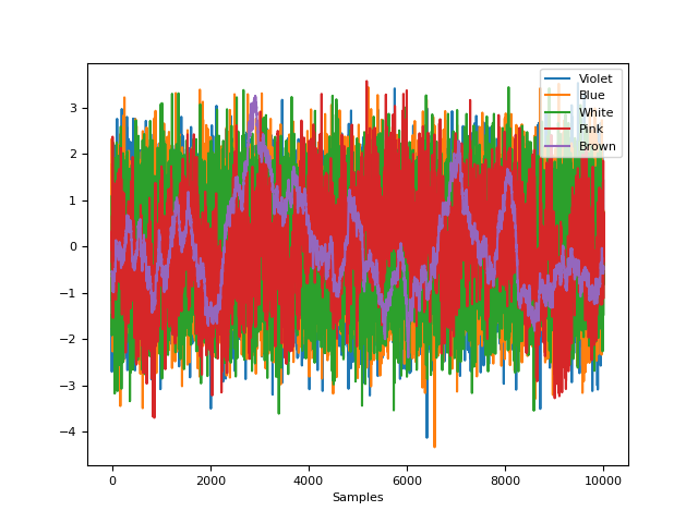
In [1]: import neurokit2 as nk

In [2]: import matplotlib.pyplot as plt

# Generate pure noise
In [3]: violet = nk.signal_noise(beta=-2)

In [4]: blue = nk.signal_noise(beta=-1)

In [5]: white = nk.signal_noise(beta=0)

In [6]: pink = nk.signal_noise(beta=1)

In [7]: brown = nk.signal_noise(beta=2)

# Visualize
In [8]: nk.signal_plot([violet, blue, white, pink, brown],
   ...:                 standardize=True,
   ...:                 labels=["Violet", "Blue", "White", "Pink", "Brown"])
   ...: 

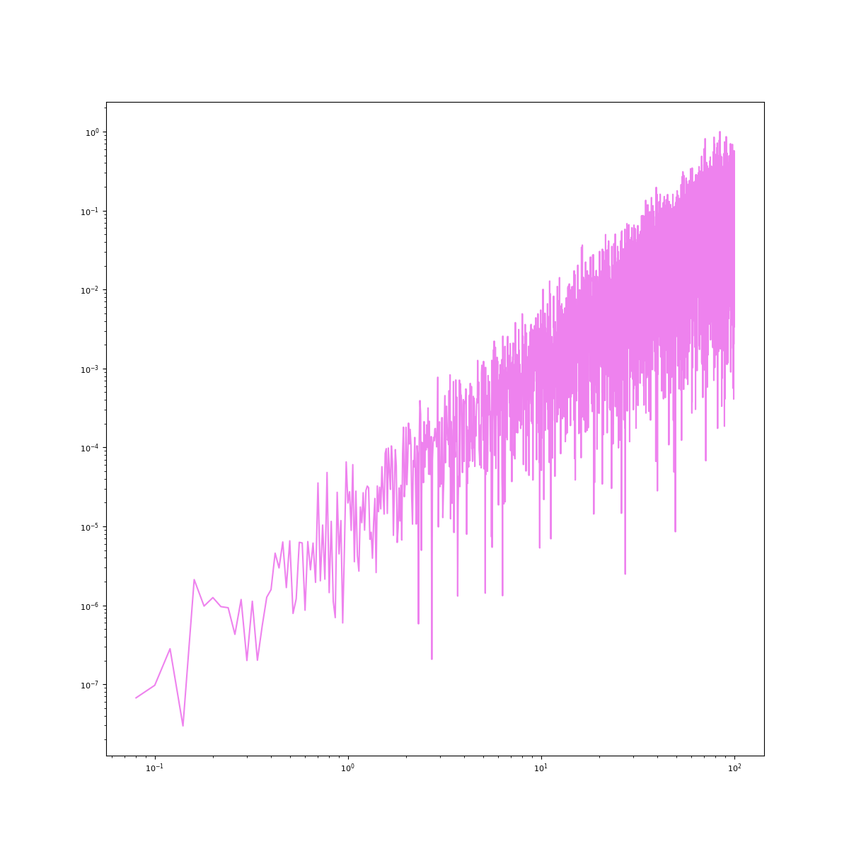
# Visualize spectrum
In [9]: psd_violet = nk.signal_psd(violet, sampling_rate=200, method="fft")

In [10]: psd_blue = nk.signal_psd(blue, sampling_rate=200, method="fft")

In [11]: psd_white = nk.signal_psd(white, sampling_rate=200, method="fft")

In [12]: psd_pink = nk.signal_psd(pink, sampling_rate=200, method="fft")

In [13]: psd_brown = nk.signal_psd(brown, sampling_rate=200, method="fft")

In [14]: plt.loglog(psd_violet["Frequency"], psd_violet["Power"], c="violet")
Out[14]: [<matplotlib.lines.Line2D at 0x255d72b2e60>]

In [15]: plt.loglog(psd_blue["Frequency"], psd_blue["Power"], c="blue")
Out[15]: [<matplotlib.lines.Line2D at 0x255c71cfa60>]

In [16]: plt.loglog(psd_white["Frequency"], psd_white["Power"], c="grey")
Out[16]: [<matplotlib.lines.Line2D at 0x255c71cffd0>]

In [17]: plt.loglog(psd_pink["Frequency"], psd_pink["Power"], c="pink")
Out[17]: [<matplotlib.lines.Line2D at 0x255c71cf430>]

In [18]: plt.loglog(psd_brown["Frequency"], psd_brown["Power"], c="brown")
Out[18]: [<matplotlib.lines.Line2D at 0x255c71cee00>]

signal_surrogate()#

signal_surrogate(signal, method='IAAFT', random_state=None, **kwargs)[source]#

Create Signal Surrogates

Generate a surrogate version of a signal. Different methods are available, such as:

random: Performs a random permutation of the signal value. This way, the signal distribution is unaffected and the serial correlations are cancelled, yielding a whitened signal with an distribution identical to that of the original.
IAAFT: Returns an Iterative Amplitude Adjusted Fourier Transform (IAAFT) surrogate. It is a phase randomized, amplitude adjusted surrogates that have the same power spectrum (to a very high accuracy) and distribution as the original data, using an iterative scheme.

Parameters:

signal (Union[list, np.array, pd.Series]) – The signal (i.e., a time series) in the form of a vector of values.
method (str) – Can be "random" or "IAAFT".
random_state (None, int, numpy.random.RandomState or numpy.random.Generator) – Seed for the random number generator. See for misc.check_random_state for further information.
**kwargs – Other keywords arguments, such as max_iter (by default 1000).

Returns:

surrogate (array) – Surrogate signal.

Examples

Create surrogates using different methods.

In [1]: import neurokit2 as nk

In [2]: import matplotlib.pyplot as plt

In [3]: signal = nk.signal_simulate(duration = 1, frequency = [3, 5], noise = 0.1)

In [4]: surrogate_iaaft = nk.signal_surrogate(signal, method = "IAAFT")

In [5]: surrogate_random = nk.signal_surrogate(signal, method = "random")

In [6]: plt.plot(surrogate_random, label = "Random Surrogate")
Out[6]: [<matplotlib.lines.Line2D at 0x255c71a1ea0>]

In [7]: plt.plot(surrogate_iaaft, label = "IAAFT Surrogate")
Out[7]: [<matplotlib.lines.Line2D at 0x255c71a2590>]

In [8]: plt.plot(signal, label = "Original")
Out[8]: [<matplotlib.lines.Line2D at 0x255c3575e70>]

In [9]: plt.legend()
Out[9]: <matplotlib.legend.Legend at 0x255c71a2230>

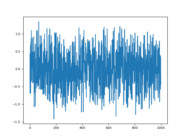
As we can see, the signal pattern is destroyed by random surrogates, but not in the IAAFT one. And their distributions are identical:

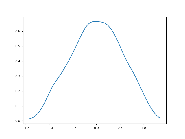
In [10]: plt.plot(*nk.density(signal), label = "Original")
Out[10]: [<matplotlib.lines.Line2D at 0x255c3597b20>]

In [11]: plt.plot(*nk.density(surrogate_iaaft), label = "IAAFT Surrogate")
Out[11]: [<matplotlib.lines.Line2D at 0x255c359ab30>]

In [12]: plt.plot(*nk.density(surrogate_random), label = "Random Surrogate")
Out[12]: [<matplotlib.lines.Line2D at 0x255c359a2f0>]

In [13]: plt.legend()
Out[13]: <matplotlib.legend.Legend at 0x255c3597d00>

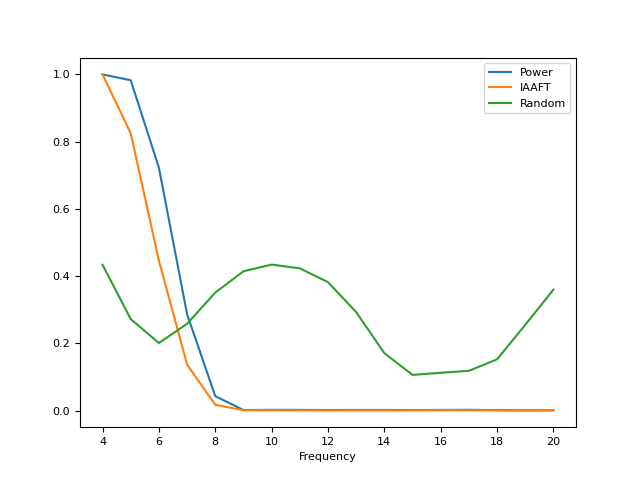
However, the power spectrum of the IAAFT surrogate is preserved.

In [14]: f = nk.signal_psd(signal, max_frequency=20)

In [15]: f["IAAFT"] = nk.signal_psd(surrogate_iaaft, max_frequency=20)["Power"]

In [16]: f["Random"] = nk.signal_psd(surrogate_random, max_frequency=20)["Power"]

In [17]: f.plot("Frequency", ["Power", "IAAFT", "Random"])
Out[17]: <Axes: xlabel='Frequency'>

References

Schreiber, T., & Schmitz, A. (1996). Improved surrogate data for nonlinearity tests. Physical review letters, 77(4), 635.

Peaks#

signal_findpeaks()#

signal_findpeaks(signal, height_min=None, height_max=None, relative_height_min=None, relative_height_max=None, relative_mean=True, relative_median=False, relative_max=False)[source]#

Find peaks in a signal

Locate peaks (local maxima) in a signal and their related characteristics, such as height (prominence), width and distance with other peaks.

Parameters:

signal (Union[list, np.array, pd.Series]) – The signal (i.e., a time series) in the form of a vector of values.
height_min (float) – The minimum height (i.e., amplitude in terms of absolute values). For example, height_min=20 will remove all peaks which height is smaller or equal to 20 (in the provided signal’s values).
height_max (float) – The maximum height (i.e., amplitude in terms of absolute values).
relative_height_min (float) – The minimum height (i.e., amplitude) relative to the sample (see below). For example, relative_height_min=-2.96 will remove all peaks which height lies below 2.96 standard deviations from the mean of the heights.
relative_height_max (float) – The maximum height (i.e., amplitude) relative to the sample (see below).
relative_mean (bool) – If a relative threshold is specified, how should it be computed (i.e., relative to what?). relative_mean=True will use Z-scores.
relative_median (bool) – If a relative threshold is specified, how should it be computed (i.e., relative to what?). Relative to median uses a more robust form of standardization (see standardize()).
relative_max (bool) – If a relative threshold is specified, how should it be computed (i.e., relative to what?). Relative to max will consider the maximum height as the reference.

Returns:

dict –

Returns a dict itself containing 5 arrays:

"Peaks": contains the peaks indices (as relative to the given signal). For instance, the value 3 means that the third data point of the signal is a peak.

"Distance": contains, for each peak, the closest distance with another peak. Note that these values will be recomputed after filtering to match the selected peaks.

"Height": contains the prominence of each peak. See scipy.signal.peak_prominences().

"Width": contains the width of each peak. See scipy.signal.peak_widths().

"Onset": contains the onset, start (or left trough), of each peak.

"Offset": contains the offset, end (or right trough), of each peak.

Examples

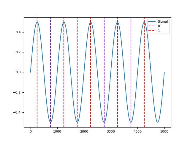
In [1]: import neurokit2 as nk

# Simulate a Signal
In [2]: signal = nk.signal_simulate(duration=5)

In [3]: info = nk.signal_findpeaks(signal)

# Visualize Onsets of Peaks and Peaks of Signal
In [4]: nk.events_plot([info["Onsets"], info["Peaks"]], signal)

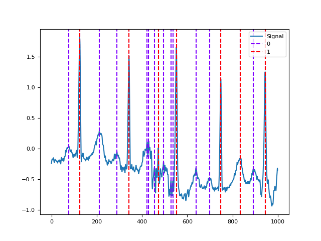
In [5]: import scipy.datasets

# Load actual ECG Signal
In [6]: ecg = scipy.datasets.electrocardiogram()

In [7]: signal = ecg[0:1000]

# Find Unfiltered and Filtered Peaks
In [8]: info1 = nk.signal_findpeaks(signal, relative_height_min=0)

In [9]: info2 = nk.signal_findpeaks(signal, relative_height_min=1)

# Visualize Peaks
In [10]: nk.events_plot([info1["Peaks"], info2["Peaks"]], signal)

See also

signal_fixpeaks

signal_fixpeaks()#

signal_fixpeaks(peaks, sampling_rate=1000, iterative=True, show=False, interval_min=None, interval_max=None, relative_interval_min=None, relative_interval_max=None, robust=False, method='Kubios', **kwargs)[source]#

Correct Erroneous Peak Placements

Identify and correct erroneous peak placements based on outliers in peak-to-peak differences (period).

Parameters:

peaks (list or array or DataFrame or Series or dict) – The samples at which the peaks occur. If an array is passed in, it is assumed that it was obtained with signal_findpeaks(). If a DataFrame is passed in, it is assumed to be obtained with ecg_findpeaks() or ppg_findpeaks() and to be of the same length as the input signal.
sampling_rate (int) – The sampling frequency of the signal that contains the peaks (in Hz, i.e., samples/second).
iterative (bool) – Whether or not to apply the artifact correction repeatedly (results in superior artifact correction).
show (bool) – Whether or not to visualize artifacts and artifact thresholds.
interval_min (float) – Only when method = "neurokit". The minimum interval between the peaks (in seconds).
interval_max (float) – Only when method = "neurokit". The maximum interval between the peaks (in seconds).
relative_interval_min (float) – Only when method = "neurokit". The minimum interval between the peaks as relative to the sample (expressed in standard deviation from the mean).
relative_interval_max (float) – Only when method = "neurokit". The maximum interval between the peaks as relative to the sample (expressed in standard deviation from the mean).
robust (bool) – Only when method = "neurokit". Use a robust method of standardization (see standardize()) for the relative thresholds.
method (str) – Either "Kubios" or "neurokit". "Kubios" uses the artifact detection and correction described in Lipponen, J. A., & Tarvainen, M. P. (2019). Note that "Kubios" is only meant for peaks in ECG or PPG. "neurokit" can be used with peaks in ECG, PPG, or respiratory data.
**kwargs – Other keyword arguments.

Returns:

peaks_clean (array) – The corrected peak locations.
artifacts (dict) – Only if method="Kubios". A dictionary containing the indices of artifacts, accessible with the keys "ectopic", "missed", "extra", and "longshort".

See also

signal_findpeaks, ecg_findpeaks, ecg_peaks, ppg_findpeaks, ppg_peaks

Examples

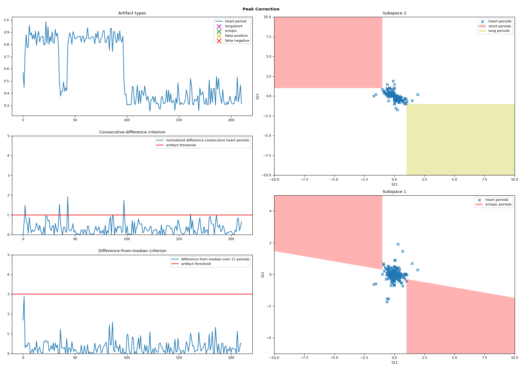
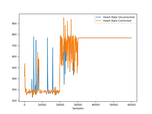
In [1]: import neurokit2 as nk

# Simulate ECG data and add noisy period
In [2]: ecg = nk.ecg_simulate(duration=240, sampling_rate=250, noise=2, random_state=42)

In [3]: ecg[20000:30000] += np.random.uniform(size=10000)

In [4]: ecg[40000:43000] = 0

# Identify and Correct Peaks using "Kubios" Method
In [5]: rpeaks_uncorrected = nk.ecg_findpeaks(ecg, method="pantompkins", sampling_rate=250)

In [6]: info, rpeaks_corrected = nk.signal_fixpeaks(
   ...:     rpeaks_uncorrected, sampling_rate=250, iterative=True, method="Kubios", show=True
   ...: )
   ...: 

# Visualize Artifact Correction
In [7]: rate_corrected = nk.signal_rate(rpeaks_corrected, desired_length=len(ecg))

In [8]: rate_uncorrected = nk.signal_rate(rpeaks_uncorrected, desired_length=len(ecg))

In [9]: nk.signal_plot(
   ...:     [rate_uncorrected, rate_corrected],
   ...:     labels=["Heart Rate Uncorrected", "Heart Rate Corrected"]
   ...: )
   ...: 

In [10]: import numpy as np

# Simulate Abnormal Signals
In [11]: signal = nk.signal_simulate(duration=4, sampling_rate=1000, frequency=1)

In [12]: peaks_true = nk.signal_findpeaks(signal)["Peaks"]

In [13]: peaks = np.delete(peaks_true, [1])  # create gaps due to missing peaks

In [14]: signal = nk.signal_simulate(duration=20, sampling_rate=1000, frequency=1)

In [15]: peaks_true = nk.signal_findpeaks(signal)["Peaks"]

In [16]: peaks = np.delete(peaks_true, [5, 15])  # create gaps

In [17]: peaks = np.sort(np.append(peaks, [1350, 11350, 18350]))  # add artifacts

# Identify and Correct Peaks using 'NeuroKit' Method
In [18]: info, peaks_corrected = nk.signal_fixpeaks(
   ....:     peaks=peaks, interval_min=0.5, interval_max=1.5, method="neurokit"
   ....: )
   ....: 

# Plot and shift original peaks to the right to see the difference.
In [19]: nk.events_plot([peaks + 50, peaks_corrected], signal)

References

Lipponen, J. A., & Tarvainen, M. P. (2019). A robust algorithm for heart rate variability time series artefact correction using novel beat classification. Journal of medical engineering & technology, 43(3), 173-181. 10.1080/03091902.2019.1640306

Analysis#

signal_autocor()#

signal_autocor(signal, lag=None, demean=True, method='auto', unbiased=False, show=False)[source]#

Autocorrelation (ACF)

Compute the autocorrelation of a signal.

Parameters:

signal (Union[list, np.array, pd.Series]) – Vector of values.
lag (int) – Time lag. If specified, one value of autocorrelation between signal with its lag self will be returned.
demean (bool) – If True, the mean of the signal will be subtracted from the signal before ACF computation.
method (str) – Using "auto" runs scipy.signal.correlate to determine the faster algorithm. Other methods are kept for legacy reasons, but are not recommended. Other methods include "correlation" (using np.correlate()) or "fft" (Fast Fourier Transform).
show (bool) – If True, plot the autocorrelation at all values of lag.

Returns:

r (float) – The cross-correlation of the signal with itself at different time lags. Minimum time lag is 0, maximum time lag is the length of the signal. Or a correlation value at a specific lag if lag is not None.
info (dict) – A dictionary containing additional information, such as the confidence interval.

Examples

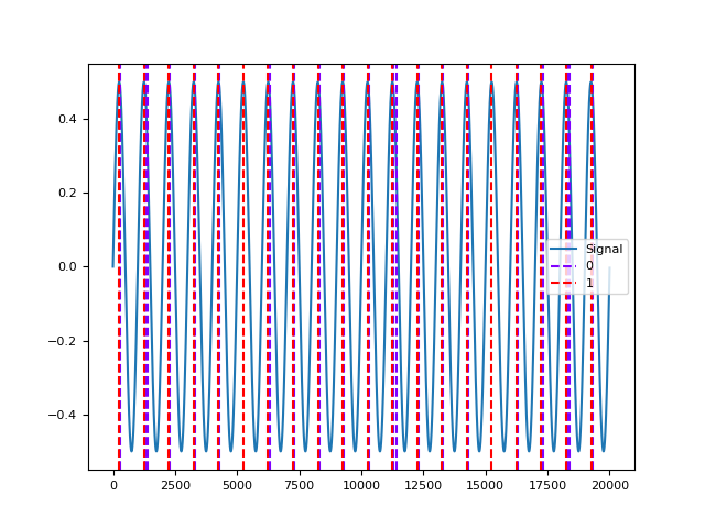
In [1]: import neurokit2 as nk

# Example 1: Using 'Correlation' Method
In [2]: signal = [1, 2, 3, 4, 5]

In [3]: r, info = nk.signal_autocor(signal, show=True, method='correlation')

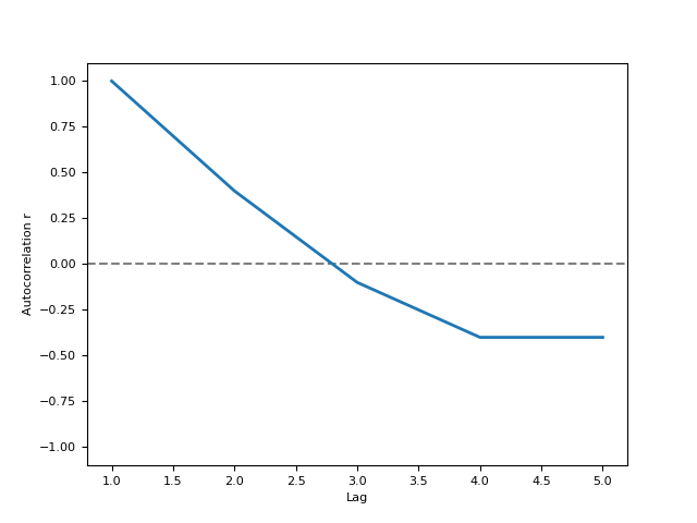
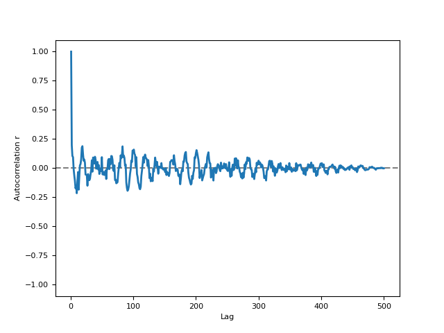
# Example 2: Using 'FFT' Method
In [4]: signal = nk.signal_simulate(duration=5, sampling_rate=100, frequency=[5, 6], noise=0.5)

In [5]: r, info = nk.signal_autocor(signal, lag=2, method='fft', show=True)

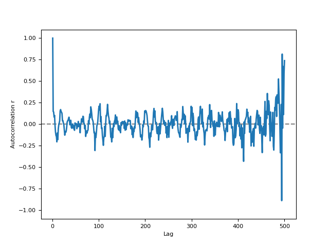
# Example 3: Using 'unbiased' Method
In [6]: r, info = nk.signal_autocor(signal, lag=2, method='fft', unbiased=True, show=True)

signal_changepoints()#

signal_changepoints(signal, change='meanvar', penalty=None, show=False)[source]#

Change Point Detection

Only the PELT method is implemented for now.

Parameters:

signal (Union[list, np.array, pd.Series]) – Vector of values.
change (str) – Can be one of "meanvar" (default), "mean" or "var".
penalty (float) – The algorithm penalty. Defaults to np.log(len(signal)).
show (bool) – Defaults to False.

Returns:

Array – Values indicating the samples at which the changepoints occur.
Fig – Figure of plot of signal with markers of changepoints.

Examples

In [1]: import neurokit2 as nk

In [2]: signal = nk.emg_simulate(burst_number=3)

In [3]: nk.signal_changepoints(signal, change="var", show=True)
Out[3]: array([1750, 2749, 3122, 3124, 4500, 5500, 7250, 8250, 9777, 9779])

References

Killick, R., Fearnhead, P., & Eckley, I. A. (2012). Optimal detection of changepoints with a linear computational cost. Journal of the American Statistical Association, 107(500), 1590-1598.

signal_period()#

signal_period(peaks, sampling_rate=1000, desired_length=None, interpolation_method='monotone_cubic')[source]#

Calculate signal period from a series of peaks

Calculate the period of a signal from a series of peaks. The period is defined as the time in seconds between two consecutive peaks.

Parameters:

peaks (Union[list, np.array, pd.DataFrame, pd.Series, dict]) – The samples at which the peaks occur. If an array is passed in, it is assumed that it was obtained with signal_findpeaks(). If a DataFrame is passed in, it is assumed it is of the same length as the input signal in which occurrences of R-peaks are marked as “1”, with such containers obtained with e.g., ecg_findpeaks() or rsp_findpeaks().
sampling_rate (int) – The sampling frequency of the signal that contains peaks (in Hz, i.e., samples/second). Defaults to 1000.
desired_length (int) – If left at the default None, the returned period will have the same number of elements as peaks. If set to a value larger than the sample at which the last peak occurs in the signal (i.e., peaks[-1]), the returned period will be interpolated between peaks over desired_length samples. To interpolate the period over the entire duration of the signal, set desired_length to the number of samples in the signal. Cannot be smaller than or equal to the sample at which the last peak occurs in the signal. Defaults to None.
interpolation_method (str) – Method used to interpolate the rate between peaks. See signal_interpolate(). "monotone_cubic" is chosen as the default interpolation method since it ensures monotone interpolation between data points (i.e., it prevents physiologically implausible “overshoots” or “undershoots” in the y-direction). In contrast, the widely used cubic spline interpolation does not ensure monotonicity.

Returns:

array – A vector containing the period.

Examples

In [1]: import neurokit2 as nk

# Generate 2 signals (with fixed and variable period)
In [2]: sig1 = nk.signal_simulate(duration=20, sampling_rate=200, frequency=1)

In [3]: sig2 = nk.ecg_simulate(duration=20, sampling_rate=200, heart_rate=60)

# Find peaks
In [4]: info1 = nk.signal_findpeaks(sig1)

In [5]: info2 = nk.ecg_findpeaks(sig2, sampling_rate=200)

# Compute period
In [6]: period1 = nk.signal_period(peaks=info1["Peaks"], desired_length=len(sig1), sampling_rate=200)

In [7]: period2 = nk.signal_period(peaks=info2["ECG_R_Peaks"], desired_length=len(sig2), sampling_rate=200)

In [8]: nk.signal_plot([period1, period2], subplots=True)

signal_phase()#

signal_phase(signal, method='radians')[source]#

Compute the phase of the signal

The real phase has the property to rotate uniformly, leading to a uniform distribution density. The prophase typically doesn’t fulfill this property. The following functions applies a nonlinear transformation to the phase signal that makes its distribution exactly uniform. If a binary vector is provided (containing 2 unique values), the function will compute the phase of completion of each phase as denoted by each value.

Parameters:

signal (Union[list, np.array, pd.Series]) – The signal (i.e., a time series) in the form of a vector of values.
method (str) – The values in which the phase is expressed. Can be "radians" (default), "degrees" (for values between 0 and 360) or "percents" (for values between 0 and 1).

Returns:: array – A vector containing the phase of the signal, between 0 and 2*pi.

Examples

In [1]: import neurokit2 as nk

In [2]: signal = nk.signal_simulate(duration=10)

In [3]: phase = nk.signal_phase(signal)

In [4]: nk.signal_plot([signal, phase])

..ipython:: python

rsp = nk.rsp_simulate(duration=30) phase = nk.signal_phase(rsp, method=”degrees”) @savefig p_signal_phase2.png scale=100% nk.signal_plot([rsp, phase]) @suppress plt.close()

# Percentage of completion of two phases
In [5]: signal = nk.signal_binarize(nk.signal_simulate(duration=10))

In [6]: phase = nk.signal_phase(signal, method="percents")

In [7]: nk.signal_plot([signal, phase])

signal_plot()#

signal_plot(signal, sampling_rate=None, subplots=False, standardize=False, labels=None, **kwargs)[source]#

Plot signal with events as vertical lines

Parameters:

signal (array or DataFrame) – Signal array (can be a dataframe with many signals).
sampling_rate (int) – The sampling frequency of the signal (in Hz, i.e., samples/second). Needs to be supplied if the data should be plotted over time in seconds. Otherwise the data is plotted over samples. Defaults to None.
subplots (bool) – If True, each signal is plotted in a subplot.
standardize (bool) – If True, all signals will have the same scale (useful for visualisation).
labels (str or list) – Defaults to None.
**kwargs (optional) – Arguments passed to matplotlib plotting.

See also

ecg_plot, rsp_plot, ppg_plot, emg_plot, eog_plot

Returns:

Though the function returns nothing, the figure can be retrieved and saved as follows
.. code-block:: console – # To be run after signal_plot() fig = plt.gcf() fig.savefig(“myfig.png”)

Examples

In [1]: import numpy as np

In [2]: import pandas as pd

In [3]: import neurokit2 as nk

In [4]: signal = nk.signal_simulate(duration=10, sampling_rate=1000)

In [5]: nk.signal_plot(signal, sampling_rate=1000, color="red")

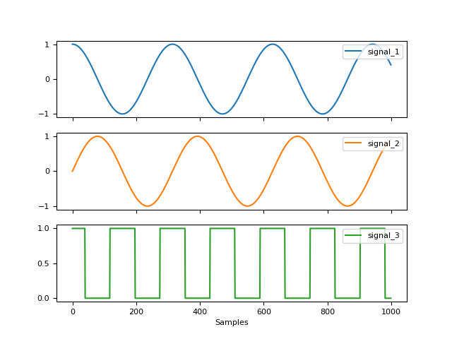
 # Simulate data
In [6]: data = pd.DataFrame({"Signal2": np.cos(np.linspace(start=0, stop=20, num=1000)),
   ...:                      "Signal3": np.sin(np.linspace(start=0, stop=20, num=1000)),
   ...:                      "Signal4": nk.signal_binarize(np.cos(np.linspace(start=0, stop=40, num=1000)))})
   ...: 

# Process signal
In [7]: nk.signal_plot(data, labels=['signal_1', 'signal_2', 'signal_3'], subplots=True)

In [8]: nk.signal_plot([signal, data], standardize=True)

signal_power()#

signal_power(signal, frequency_band, sampling_rate=1000, continuous=False, show=False, normalize=True, **kwargs)[source]#

Compute the power of a signal in a given frequency band

Parameters:

signal (Union[list, np.array, pd.Series]) – The signal (i.e., a time series) in the form of a vector of values.
frequency_band (tuple or list) – Tuple or list of tuples indicating the range of frequencies to compute the power in.
sampling_rate (int) – The sampling frequency of the signal (in Hz, i.e., samples/second).
continuous (bool) – Compute instant frequency, or continuous power.
show (bool) – If True, will return a Poincaré plot. Defaults to False.
normalize (bool) – Normalization of power by maximum PSD value. Default to True. Normalization allows comparison between different PSD methods.
**kwargs – Keyword arguments to be passed to signal_psd().

See also

signal_filter, signal_psd

Returns:: pd.DataFrame – A DataFrame containing the Power Spectrum values and a plot if show is True.

Examples

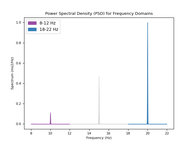
In [1]: import neurokit2 as nk

In [2]: import numpy as np

# Instant power
In [3]: signal = nk.signal_simulate(duration=60, frequency=[10, 15, 20],
   ...:                             amplitude = [1, 2, 3], noise = 2)
   ...: 

In [4]: power_plot = nk.signal_power(signal, frequency_band=[(8, 12), (18, 22)], method="welch", show=True)

..ipython:: python

# Continuous (simulated signal) signal = np.concatenate((nk.ecg_simulate(duration=30, heart_rate=75), nk.ecg_simulate(duration=30, heart_rate=85))) power = nk.signal_power(signal, frequency_band=[(72/60, 78/60), (82/60, 88/60)], continuous=True) processed, _ = nk.ecg_process(signal) power[“ECG_Rate”] = processed[“ECG_Rate”]

@savefig p_signal_power2.png scale=100% nk.signal_plot(power, standardize=True) @suppress plt.close()

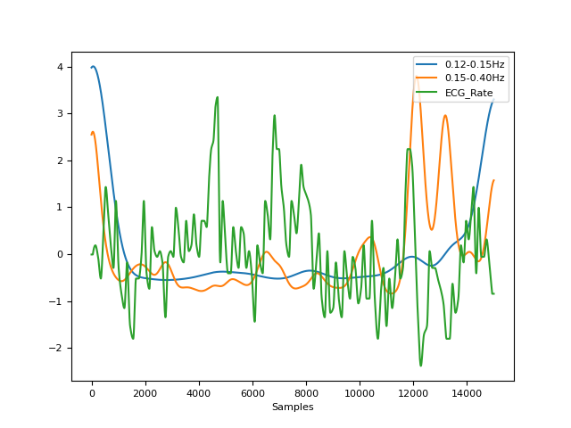
# Continuous (real signal)
In [5]: signal = nk.data("bio_eventrelated_100hz")["ECG"]

In [6]: power = nk.signal_power(signal, sampling_rate=100, frequency_band=[(0.12, 0.15), (0.15, 0.4)], continuous=True)

In [7]: processed, _ = nk.ecg_process(signal, sampling_rate=100)

In [8]: power["ECG_Rate"] = processed["ECG_Rate"]

In [9]: nk.signal_plot(power, standardize=True)

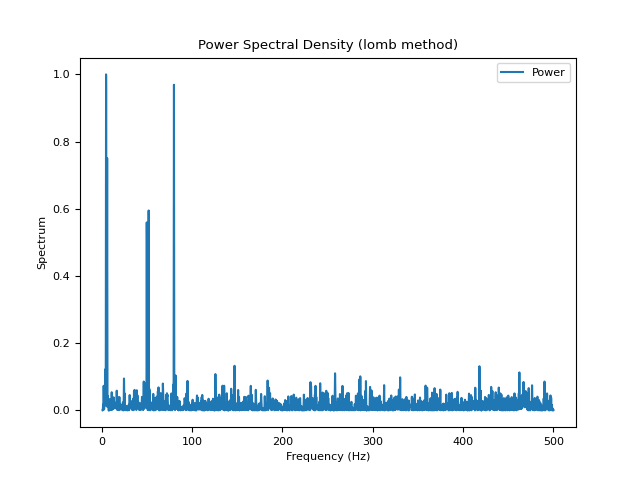
signal_psd()#

signal_psd(signal, sampling_rate=1000, method='welch', show=False, normalize=True, min_frequency='default', max_frequency=inf, window=None, window_type='hann', order=16, order_criteria='KIC', order_corrected=True, silent=True, t=None, **kwargs)[source]#

Compute the Power Spectral Density (PSD)

Parameters:

signal (Union[list, np.array, pd.Series]) – The signal (i.e., a time series) in the form of a vector of values.
sampling_rate (int) – The sampling frequency of the signal (in Hz, i.e., samples/second).
method (str) – Either "welch" (default), "fft", "multitapers" (requires the ‘mne’ package), "lombscargle" (requires the ‘astropy’ package) or "burg".
show (bool) – If True, will return a plot. If False, will return the density values that can be plotted externally.
normalize (bool) – Normalization of power by maximum PSD value. Default to True. Normalization allows comparison between different PSD methods.
min_frequency (str, float) – The minimum frequency. If default, min_frequency is chosen based on the sampling rate and length of signal to optimize the frequency resolution.
max_frequency (float) – The maximum frequency.
window (int) – Length of each window in seconds (for “Welch” method). If None (default), window will be automatically calculated to capture at least 2 cycles of min_frequency. If the length of recording does not allow the formal, window will be default to half of the length of recording.
window_type (str) – Desired window to use. Defaults to "hann". See scipy.signal.get_window() for list of windows.
order (int) – The order of autoregression (only used for autoregressive (AR) methods such as "burg").
order_criteria (str) – The criteria to automatically select order in parametric PSD (only used for autoregressive (AR) methods such as "burg").
order_corrected (bool) – Should the order criteria (AIC or KIC) be corrected? If unsure which method to use to choose the order, rely on the default (i.e., the corrected KIC).
silent (bool) – If False, warnings will be printed. Default to True.
t (array) – The timestamps corresponding to each sample in the signal, in seconds (for "lombscargle" method). Defaults to None.
**kwargs (optional) – Keyword arguments to be passed to scipy.signal.welch().

See also

signal_filter, mne.time_frequency.psd_array_multitaper, scipy.signal.welch

Returns:: data (pd.DataFrame) – A DataFrame containing the Power Spectrum values and a plot if show is True.

Examples

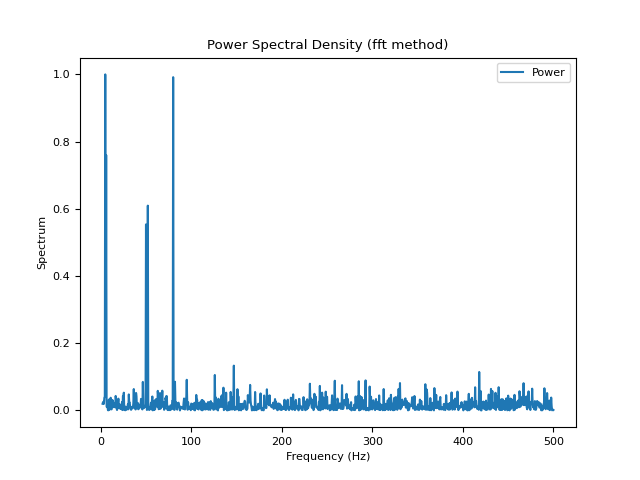
In [1]: import neurokit2 as nk

In [2]: signal = nk.signal_simulate(duration=2, frequency=[5, 6, 50, 52, 80], noise=0.5)

# FFT method (based on numpy)
In [3]: psd_multitapers = nk.signal_psd(signal, method="fft", show=True)

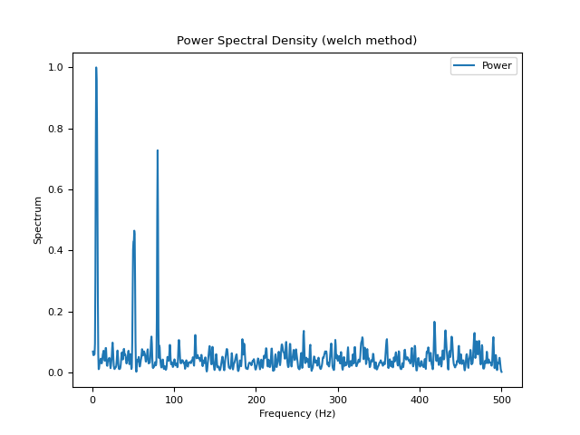
# Welch method (based on scipy)
In [4]: psd_welch = nk.signal_psd(signal, method="welch", min_frequency=1, show=True)

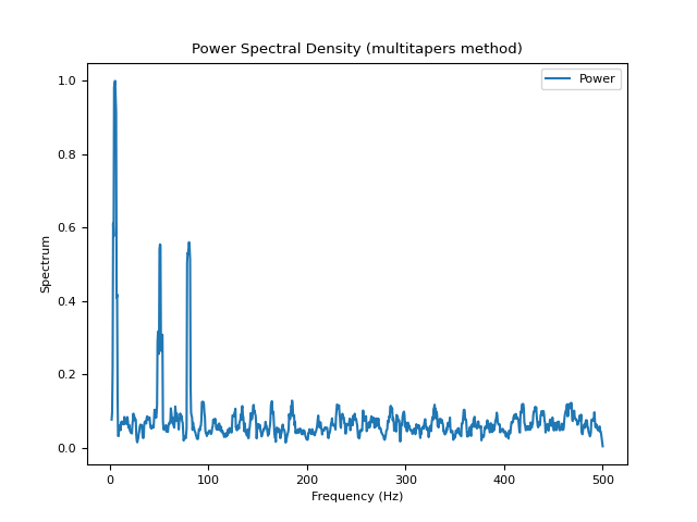
# Multitapers method (requires MNE)
In [5]: psd_multitapers = nk.signal_psd(signal, method="multitapers", show=True)

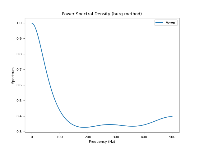
# Burg method
In [6]: psd_burg = nk.signal_psd(signal, method="burg", min_frequency=1, show=True)

# Lomb method (requires AstroPy)
In [7]: psd_lomb = nk.signal_psd(signal, method="lomb", min_frequency=1, show=True)

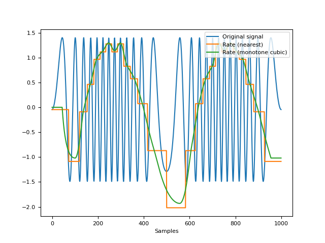
signal_rate()#

signal_rate(peaks, sampling_rate=1000, desired_length=None, interpolation_method='monotone_cubic', show=False)[source]#

Compute Signal Rate

Calculate signal rate (per minute) from a series of peaks. It is a general function that works for any series of peaks (i.e., not specific to a particular type of signal). It is computed as 60 / period, where the period is the time between the peaks (see func:.signal_period).

Note

This function is implemented under signal_rate(), but it also re-exported under different names, such as ecg_rate(), or rsp_rate(). The aliases are provided for consistency.

Parameters:

peaks (Union[list, np.array, pd.DataFrame, pd.Series, dict]) – The samples at which the peaks occur. If an array is passed in, it is assumed that it was obtained with signal_findpeaks(). If a DataFrame is passed in, it is assumed it is of the same length as the input signal in which occurrences of R-peaks are marked as “1”, with such containers obtained with e.g., :func:.`ecg_findpeaks` or rsp_findpeaks().
sampling_rate (int) – The sampling frequency of the signal that contains peaks (in Hz, i.e., samples/second). Defaults to 1000.
desired_length (int) – If left at the default None, the returned rated will have the same number of elements as peaks. If set to a value larger than the sample at which the last peak occurs in the signal (i.e., peaks[-1]), the returned rate will be interpolated between peaks over desired_length samples. To interpolate the rate over the entire duration of the signal, set desired_length to the number of samples in the signal. Cannot be smaller than or equal to the sample at which the last peak occurs in the signal. Defaults to None.
interpolation_method (str) – Method used to interpolate the rate between peaks. See signal_interpolate().
"monotone_cubic" is chosen as the default interpolation method since it ensures monotone interpolation between data points (i.e., it prevents physiologically implausible “overshoots” or “undershoots” in the y-direction). In contrast, the widely used cubic spline interpolation does not ensure monotonicity.

showbool
If True, shows a plot. Defaults to False.

Returns:

array – A vector containing the rate (peaks per minute).

Examples

In [8]: import neurokit2 as nk

# Create signal of varying frequency
In [9]: freq = nk.signal_simulate(1, frequency = 1)

In [10]: signal = np.sin((freq).cumsum() * 0.5)

# Find peaks
In [11]: info = nk.signal_findpeaks(signal)

# Compute rate using 2 methods
In [12]: rate1 = nk.signal_rate(peaks=info["Peaks"],
   ....:                        desired_length=len(signal),
   ....:                        interpolation_method="nearest")
   ....: 

In [13]: rate2 = nk.signal_rate(peaks=info["Peaks"],
   ....:                        desired_length=len(signal),
   ....:                        interpolation_method="monotone_cubic")
   ....: 

# Visualize signal and rate on the same scale
In [14]: nk.signal_plot([signal, rate1, rate2],
   ....:                labels = ["Original signal", "Rate (nearest)", "Rate (monotone cubic)"],
   ....:                standardize = True)
   ....: 

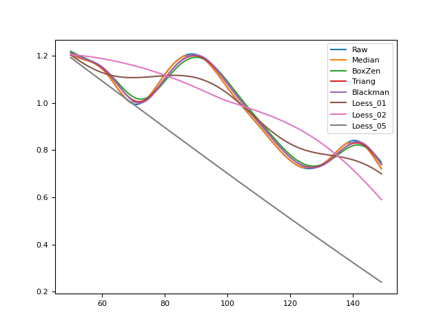
signal_smooth()#

signal_smooth(signal, method='convolution', kernel='boxzen', size=10, alpha=0.1)[source]#

Signal smoothing

Signal smoothing can be achieved using either the convolution of a filter kernel with the input signal to compute the smoothed signal (Smith, 1997) or a LOESS regression.

Parameters:

signal (Union[list, np.array, pd.Series]) – The signal (i.e., a time series) in the form of a vector of values.
method (str) – Can be one of "convolution" (default) or "loess".
kernel (Union[str, np.array]) – Only used if method is "convolution". Type of kernel to use; if array, use directly as the kernel. Can be one of "median", "boxzen", "boxcar", "triang", "blackman", "hamming", "hann", "bartlett", "flattop", "parzen", "bohman", "blackmanharris", "nuttall", "barthann", "kaiser" (needs beta), "gaussian" (needs std), "general_gaussian" (needs power width), "slepian" (needs width) or "chebwin" (needs attenuation).
size (int) – Only used if method is "convolution". Size of the kernel; ignored if kernel is an array.
alpha (float) – Only used if method is "loess". The parameter which controls the degree of smoothing.

Returns:

array – Smoothed signal.

See also

fit_loess

Examples

In [1]: import numpy as np

In [2]: import pandas as pd

In [3]: import neurokit2 as nk

In [4]: signal = np.cos(np.linspace(start=0, stop=10, num=1000))

In [5]: distorted = nk.signal_distort(signal,
   ...:                               noise_amplitude=[0.3, 0.2, 0.1, 0.05],
   ...:                               noise_frequency=[5, 10, 50, 100])
   ...: 

In [6]: size = len(signal)/100

In [7]: signals = pd.DataFrame({"Raw": distorted,
   ...:                         "Median": nk.signal_smooth(distorted, kernel="median", size=size-1),
   ...:                         "BoxZen": nk.signal_smooth(distorted, kernel="boxzen", size=size),
   ...:                         "Triang": nk.signal_smooth(distorted, kernel="triang", size=size),
   ...:                         "Blackman": nk.signal_smooth(distorted, kernel="blackman", size=size),
   ...:                         "Loess_01": nk.signal_smooth(distorted, method="loess", alpha=0.1),
   ...:                         "Loess_02": nk.signal_smooth(distorted, method="loess", alpha=0.2),
   ...:                         "Loess_05": nk.signal_smooth(distorted, method="loess", alpha=0.5)})
   ...: 

In [8]: fig = signals.plot()

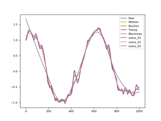
# Magnify the plot
In [9]: fig_magnify = signals[50:150].plot()

References

Smith, S. W. (1997). The scientist and engineer’s guide to digital signal processing.

signal_synchrony()#

signal_synchrony(signal1, signal2, method='hilbert', window_size=50)[source]#

Synchrony (coupling) between two signals

Signal coherence refers to the strength of the mutual relationship (i.e., the amount of shared information) between two signals. Synchrony is coherence “in phase” (two waveforms are “in phase” when the peaks and troughs occur at the same time). Synchrony will always be coherent, but coherence need not always be synchronous.

This function computes a continuous index of coupling between two signals either using the "hilbert" method to get the instantaneous phase synchrony, or using a rolling window correlation.

The instantaneous phase synchrony measures the phase similarities between signals at each timepoint. The phase refers to the angle of the signal, calculated through the hilbert transform, when it is resonating between -pi to pi degrees. When two signals line up in phase their angular difference becomes zero.

For less clean signals, windowed correlations are widely used because of their simplicity, and can be a good a robust approximation of synchrony between two signals. The limitation is the need to select a window size.

Parameters:

signal1 (Union[list, np.array, pd.Series]) – Time series in the form of a vector of values.
signal2 (Union[list, np.array, pd.Series]) – Time series in the form of a vector of values.
method (str) – The method to use. Can be one of "hilbert" or "correlation".
window_size (int) – Only used if method='correlation'. The number of samples to use for rolling correlation.

See also

scipy.signal.hilbert, mutual_information

Returns:: array – A vector containing the phase of the signal, between 0 and 2*pi.

Examples

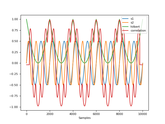
In [1]: import neurokit2 as nk

In [2]: s1 = nk.signal_simulate(duration=10, frequency=1)

In [3]: s2 = nk.signal_simulate(duration=10, frequency=1.5)

In [4]: coupling1 = nk.signal_synchrony(s1, s2, method="hilbert")

In [5]: coupling2 = nk.signal_synchrony(s1, s2, method="correlation", window_size=1000/2)

In [6]: nk.signal_plot([s1, s2, coupling1, coupling2], labels=["s1", "s2", "hilbert", "correlation"])

References

http://jinhyuncheong.com/jekyll/update/2017/12/10/Timeseries_synchrony_tutorial_and_simulations.html

signal_timefrequency()#

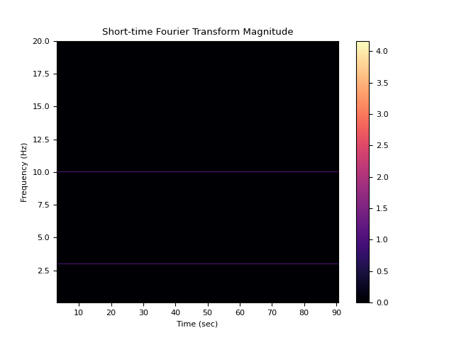
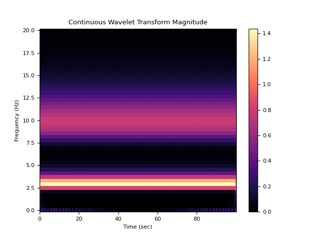
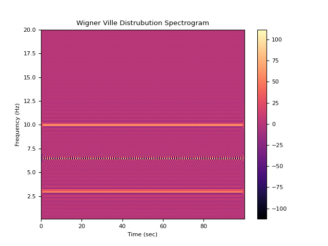
signal_timefrequency(signal, sampling_rate=1000, min_frequency=0.04, max_frequency=None, method='stft', window=None, window_type='hann', mode='psd', nfreqbin=None, overlap=None, analytical_signal=True, show=True)[source]#

Quantify changes of a nonstationary signal’s frequency over time The objective of time-frequency analysis is to offer a more informative description of the signal which reveals the temporal variation of its frequency contents.

There are many different Time-Frequency Representations (TFRs) available:

Linear TFRs: efficient but create tradeoff between time and frequency resolution
- Short Time Fourier Transform (STFT): the time-domain signal is windowed into short segments and FT is applied to each segment, mapping the signal into the TF plane. This method assumes that the signal is quasi-stationary (stationary over the duration of the window). The width of the window is the trade-off between good time (requires short duration window) versus good frequency resolution (requires long duration windows)
- Wavelet Transform (WT): similar to STFT but instead of a fixed duration window function, a varying window length by scaling the axis of the window is used. At low frequency, WT proves high spectral resolution but poor temporal resolution. On the other hand, for high frequencies, the WT provides high temporal resolution but poor spectral resolution.
Quadratic TFRs: better resolution but computationally expensive and suffers from having cross terms between multiple signal components
- Wigner Ville Distribution (WVD): while providing very good resolution in time and frequency of the underlying signal structure, because of its bilinear nature, existence of negative values, the WVD has misleading TF results in the case of multi-component signals such as EEG due to the presence of cross terms and inference terms. Cross WVD terms can be reduced by using smoothing kernel functions as well as analyzing the analytic signal (instead of the original signal)
- Smoothed Pseudo Wigner Ville Distribution (SPWVD): to address the problem of cross-terms suppression, SPWVD allows two independent analysis windows, one in time and the other in frequency domains.

Parameters:

signal (Union[list, np.array, pd.Series]) – The signal (i.e., a time series) in the form of a vector of values.
sampling_rate (int) – The sampling frequency of the signal (in Hz, i.e., samples/second).
method (str) – Time-Frequency decomposition method.
min_frequency (float) – The minimum frequency.
max_frequency (float) – The maximum frequency.
window (int) – Length of each segment in seconds. If None (default), window will be automatically calculated. For "STFT" method.
window_type (str) – Type of window to create, defaults to "hann". See scipy.signal.get_window() to see full options of windows. For "STFT" method.
mode (str) – Type of return values for "STFT" method. Can be "psd", "complex" (default, equivalent to output of "STFT" with no padding or boundary extension), "magnitude", "angle", "phase". Defaults to "psd".
nfreqbin (int, float) – Number of frequency bins. If None (default), nfreqbin will be set to 0.5*sampling_rate.
overlap (int) – Number of points to overlap between segments. If None, noverlap = nperseg // 8. Defaults to None.
analytical_signal (bool) – If True, analytical signal instead of actual signal is used in Wigner Ville Distribution methods.
show (bool) – If True, will return two PSD plots.

Returns:

frequency (np.array) – Frequency.
time (np.array) – Time array.
stft (np.array) – Short Term Fourier Transform. Time increases across its columns and frequency increases down the rows.

Examples

In [1]: import neurokit2 as nk

In [2]: sampling_rate = 100

In [3]: signal = nk.signal_simulate(100, sampling_rate, frequency=[3, 10])

# STFT Method
In [4]: f, t, stft = nk.signal_timefrequency(signal,
   ...:                                      sampling_rate,
   ...:                                      max_frequency=20,
   ...:                                      method="stft",
   ...:                                      show=True)
   ...: 

# CWTM Method
In [5]: f, t, cwtm = nk.signal_timefrequency(signal,
   ...:                                      sampling_rate,
   ...:                                      max_frequency=20,
   ...:                                      method="cwt",
   ...:                                      show=True)
   ...: 

# WVD Method
In [6]: f, t, wvd = nk.signal_timefrequency(signal,
   ...:                                     sampling_rate,
   ...:                                     max_frequency=20,
   ...:                                     method="wvd",
   ...:                                     show=True)
   ...: 

# PWVD Method
In [7]: f, t, pwvd = nk.signal_timefrequency(signal,
   ...:                                      sampling_rate,
   ...:                                      max_frequency=20,
   ...:                                      method="pwvd",
   ...:                                      show=True)
   ...: 

signal_zerocrossings()#

signal_zerocrossings(signal, direction='both')[source]#

Locate the indices where the signal crosses zero

Note that when the signal crosses zero between two points, the first index is returned.

Parameters:

signal (Union[list, np.array, pd.Series]) – The signal (i.e., a time series) in the form of a vector of values.
direction (str) – Direction in which the signal crosses zero, can be "positive", "negative" or "both" (default).

Returns:

array – Vector containing the indices of zero crossings.

Examples

In [1]: import neurokit2 as nk

In [2]: signal = nk.signal_simulate(duration=5)

In [3]: zeros = nk.signal_zerocrossings(signal)

In [4]: nk.events_plot(zeros, signal)

# Only upward or downward zerocrossings
In [5]: up = nk.signal_zerocrossings(signal, direction="up")

In [6]: down = nk.signal_zerocrossings(signal, direction="down")

In [7]: nk.events_plot([up, down], signal)

Any function appearing below this point is not explicitly part of the documentation and should be added. Please open an issue if there is one.

Submodule for NeuroKit.

signal_fillmissing(signal, method='both')[source]#

Handle missing values

Fill missing values in a signal using specific methods.

Parameters:

signal (Union[list, np.array, pd.Series]) – The signal (i.e., a time series) in the form of a vector of values.
method (str) – The method to use to fill missing values. Can be one of "forward", "backward", or "both". The default is "both".

Returns:

signal

Examples

In [1]: import neurokit2 as nk

In [2]: signal = [np.nan, 1, 2, 3, np.nan, np.nan, 6, 7, np.nan]

In [3]: nk.signal_fillmissing(signal, method="forward")
Out[3]: array([nan,  1.,  2.,  3.,  3.,  3.,  6.,  7.,  7.])

In [4]: nk.signal_fillmissing(signal, method="backward")
Out[4]: array([ 1.,  1.,  2.,  3.,  6.,  6.,  6.,  7., nan])

In [5]: nk.signal_fillmissing(signal, method="both")
Out[5]: array([1., 1., 2., 3., 3., 3., 6., 7., 7.])

signal_formatpeaks(info, desired_length, peak_indices=None, other_indices=None)[source]#

Format Peaks

Transforms a peak-info dict to a signal of given length

Signal Processing

Contents

Signal Processing#

Preprocessing#

signal_simulate()#

signal_filter()#

signal_sanitize()#

signal_resample()#

signal_fillmissing()#

Transformation#

signal_binarize()#

signal_decompose()#

signal_recompose()#

signal_detrend()#

signal_distort()#

signal_flatline()#

signal_interpolate()#

signal_merge()#

signal_noise()#

signal_surrogate()#

Peaks#

signal_findpeaks()#

signal_fixpeaks()#

Analysis#

signal_autocor()#

signal_changepoints()#

signal_period()#

signal_phase()#

signal_plot()#

signal_power()#

signal_psd()#

signal_rate()#

signal_smooth()#

signal_synchrony()#

signal_timefrequency()#

signal_zerocrossings()#