Analyze Electrodermal Activity (EDA)#
This example can be referenced by citing the package.
This example shows how to use NeuroKit2 to extract the features from Electrodermal Activity (EDA).
# Load the NeuroKit package
import neurokit2 as nk
Extract the cleaned EDA signal#
In this example, we will use a simulated EDA signal. However, you can use any signal you have generated (for instance, extracted from the dataframe using read_acqknowledge().
# Simulate 10 seconds of EDA Signal (recorded at 250 samples / second)
eda_signal = nk.eda_simulate(duration=10, sampling_rate=250, scr_number=3, drift=0.01)
Once you have a raw EDA signal in the shape of a vector (i.e., a one-dimensional array), or a list, you can use eda_process() to process it.
# Process the raw EDA signal
signals, info = nk.eda_process(eda_signal, sampling_rate=250)
Note: It is critical that you specify the correct sampling rate of your signal throughout many processing functions, as this allows NeuroKit to have a time reference.
This function outputs two elements, a dataframe containing the different signals (e.g., the raw signal, clean signal, SCR samples marking the different features etc.), and a dictionary containing information about the Skin Conductance Response (SCR) peaks (e.g., onsets, peak amplitude etc.).
Locate Skin Conductance Response (SCR) features#
The processing function does two important things for our purpose: Firstly, it cleans the signal. Secondly, it detects the location of 1) peak onsets, 2) peak amplitude, and 3) half-recovery time. Let’s extract these from the output.
# Extract clean EDA and SCR features
cleaned = signals["EDA_Clean"]
features = [info["SCR_Onsets"], info["SCR_Peaks"], info["SCR_Recovery"]]
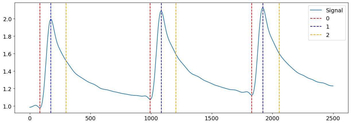
We can now visualize the location of the peak onsets, the peak amplitude, as well as the half-recovery time points in the cleaned EDA signal, respectively marked by the red dashed line, blue dashed line, and orange dashed line.
# Visualize SCR features in cleaned EDA signal
plot = nk.events_plot(features, cleaned, color=["red", "blue", "orange"])
Decompose EDA into Phasic and Tonic components#
We can also decompose the EDA signal into its phasic and tonic components, or more specifically, the Phasic Skin Conductance Response (SCR) and the Tonic Skin Conductance Level (SCL) respectively. The SCR represents the stimulus-dependent fast changing signal whereas the SCL is slow-changing and continuous. Separating these two signals helps to provide a more accurate estimation of the true SCR amplitude.
# Filter phasic and tonic components
data = nk.eda_phasic(nk.standardize(eda_signal), sampling_rate=250)
Note: here we standardized the raw EDA signal before the decomposition, which can be useful in the presence of high inter-individual variations.
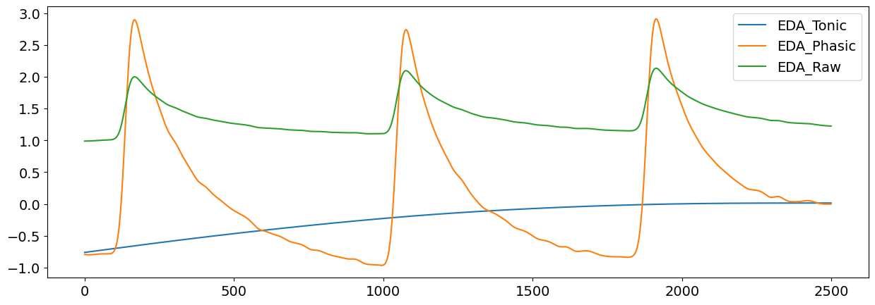
We can now add the raw signal to the dataframe containing the two signals, and plot them!
data["EDA_Raw"] = eda_signal  # Add raw signal
data.plot()
<Axes: >
Quick Plot#
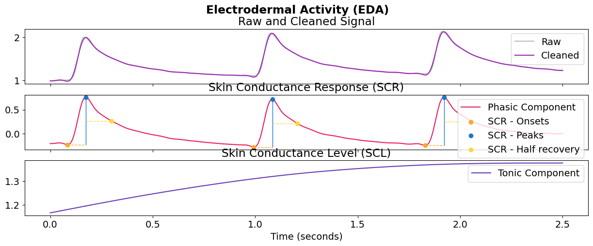
You can obtain all of these features by using the eda_plot() function on the dataframe of processed EDA.
# Plot EDA signal
nk.eda_plot(signals)
/home/runner/work/NeuroKit/NeuroKit/neurokit2/eda/eda_plot.py:49: NeuroKitWarning: 'info' dict not provided. Some information might be missing. Sampling rate will be set to 1000 Hz.
  warn(