Fit a function to a non-linear pattern

This example can be referenced by citing the package.

This small tutorial will show you how to use Python to estimate the best fitting line to some data. This can be used to find the optimal line passing through a signal.

# Load NeuroKit and other useful packages
import neurokit2 as nk
import pandas as pd
import numpy as np
import scipy.optimize
import matplotlib.pyplot as plt

Fit a linear function

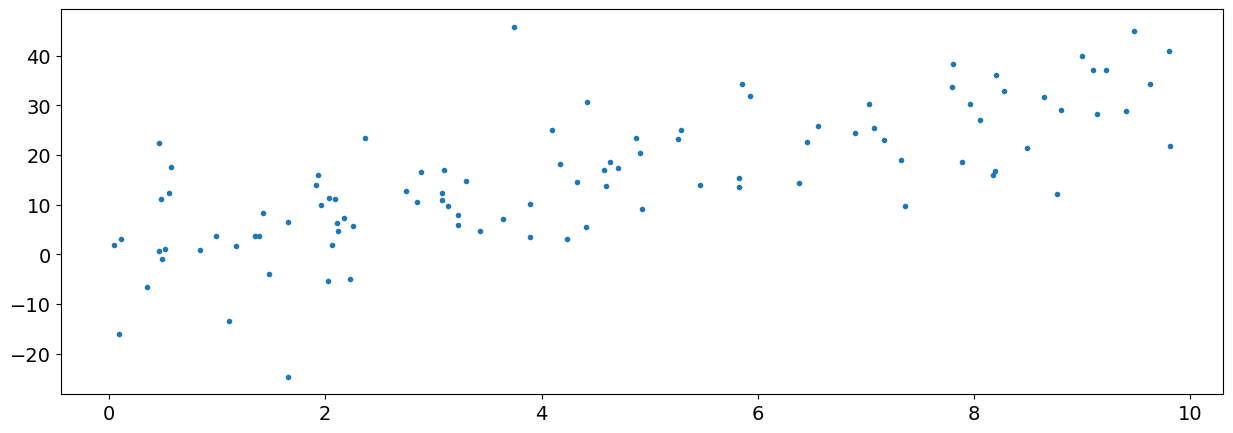
We will start by generating some random data on a scale from 0 to 10 (the x-axis), and then pass them through a function to create its y values.

x = np.random.uniform(0., 10., size=100)
y = 3. * x + 2. + np.random.normal(0., 10., 100)
plt.plot(x, y, '.')
plt.show()

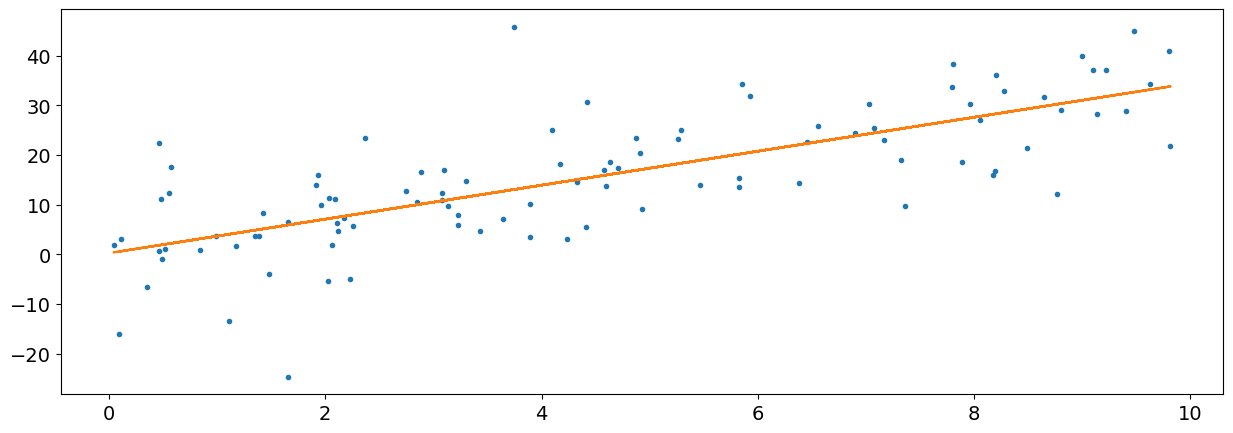
In this case we know that the best fitting line will be a linear function (i.e., a straight line), and we want to find its parameters. A linear function has two parameters, the intercept and the slope.

First, we need to create this function, that takes some x values, the parameters, and return the y value.

def function_linear(x, intercept, slope):
    y =  intercept + slope * x
    return y

Now, using the power of scipy, we can optimize this function based on our data to find the parameters that minimize the least square error. It just needs the function and the data’s x and y values.

params, covariance = scipy.optimize.curve_fit(function_linear, x, y)
params

array([-0.49757261,  3.42423923])

So the optimal parameters (in our case, the intercept and the slope) are returned in the params object. We can unpack these parameters (using the star symbol *) into our linear function to use them, and create the predicted y values to our x axis.

fit = function_linear(x, *params)

plt.plot(x, y, '.')
plt.plot(x, fit, '-')
plt.show()

Non-linear curves

We can also use that to approximate non-linear curves.

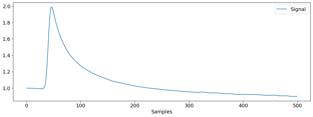
signal = nk.eda_simulate(sampling_rate=50)
nk.signal_plot(signal)

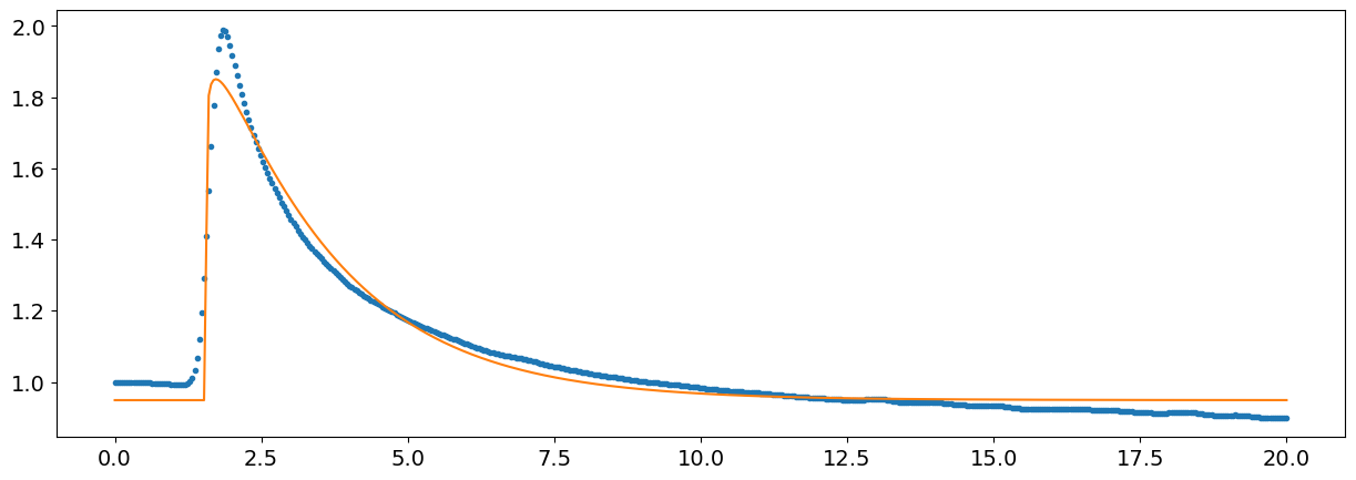
In this example, we will try to approximate this Skin Conductance Response (SCR) using a gamma distribution, which is quite a flexible distribution defined by 3 parameters (a, loc and scale).

On top of these 3 parameters, we will add 2 more, the intercept and a size parameter to give it more flexibility.

def function_gamma(x, intercept, size, a, loc, scale):
    gamma = scipy.stats.gamma.pdf(x, a=a, loc=loc, scale=scale)
    y = intercept + (size * gamma)
    return y

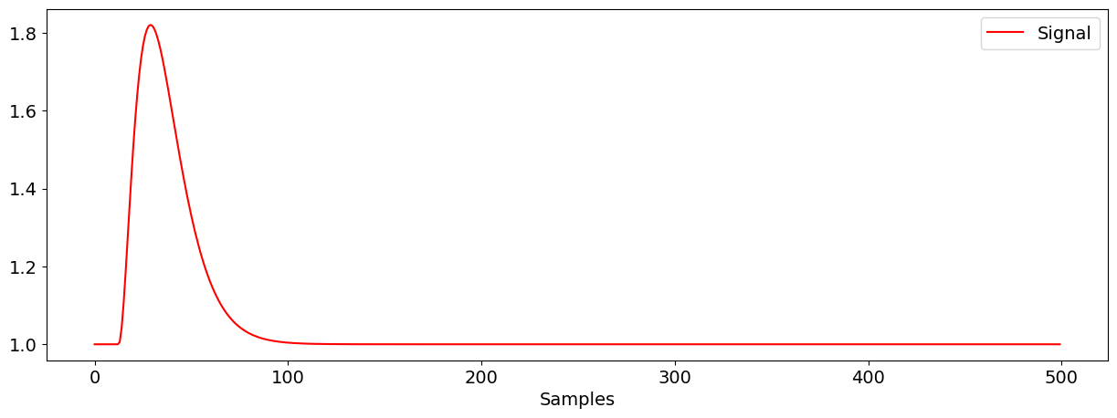
We can start by visualizing the function with a “arbitrary” parameters:

x = np.linspace(0, 20, num=500)
y = function_gamma(x, intercept=1, size=1, a=3, loc=0.5, scale=0.33)

nk.signal_plot(y, color="red")

Since these values are already a good start, we will use them as “starting point” (through the p0 argument), to help the estimation algorithm converge (otherwise it could never find the right combination of parameters).

params, covariance = scipy.optimize.curve_fit(function_gamma, x, signal, p0=[1, 1, 3, 0.5, 0.33])
params

array([0.94633497, 2.31509615, 1.03768108, 1.16232463, 2.12672397])

fit = function_gamma(x, *params)

plt.plot(x, signal, '.')
plt.plot(x, fit, '-')
plt.show()