EEG Complexity Analysis

In this example, we are going to apply complexity analysis to EEG data. Useful reads include:

• List of complexity indices available in NeuroKit

• EEG Complexity review (Lau et al., 2022)

• What complexity indices to select (Makowski et al., 2022)

This example below can be referenced by citing the package.

# Load packages
import numpy as np
import pandas as pd
import matplotlib.pyplot as plt
import seaborn as sns
import scipy.stats
import mne
import neurokit2 as nk

Data Preprocessing

Load and format the EEG data of one participant following this MNE example.

# Load raw EEG data
raw = nk.data("eeg_1min_200hz")

# Find events and map them to a condition (for event-related analysis)
events = mne.find_events(raw, stim_channel='STI 014', verbose=False)
event_dict = {'auditory/left': 1, 'auditory/right': 2, 'visual/left': 3,
              'visual/right': 4, 'face': 5, 'buttonpress': 32}

# Select only relevant channels
raw = raw.pick('eeg', verbose=False)

# Store sampling rate
sampling_rate = raw.info["sfreq"]

raw = raw.filter(l_freq=0.1, h_freq=40,verbose=False)
fig = raw.plot_sensors(show_names=True)

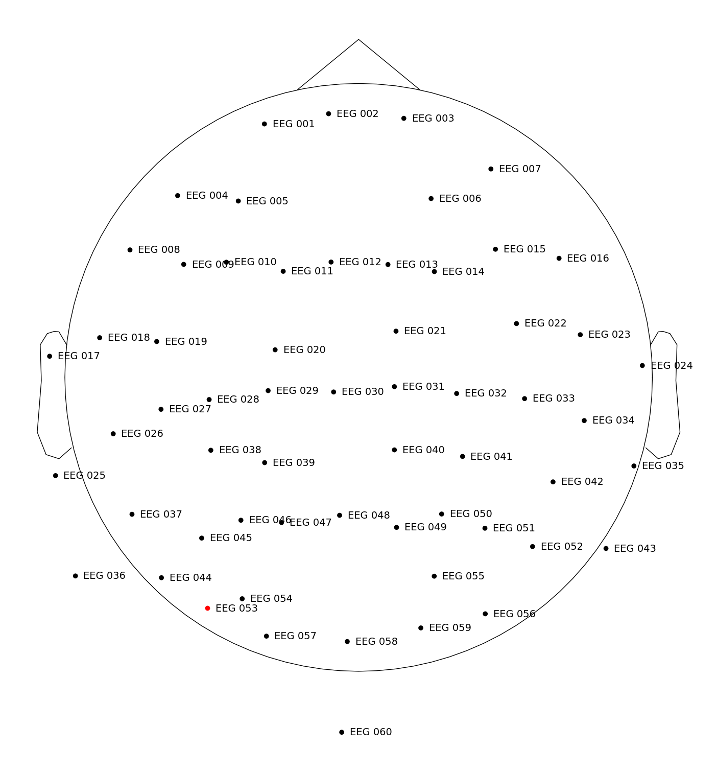
Interval-related Complexity Analysis

This type of analysis is suited for when we don’t have time-locked “events”, and we want to compute the complexity over the whole signal (e.g., in resting-state paradigms).

We will first extract the signal at a subset of channels of interest (region of interest, ROI). We will pick 4 fronto-central channels, namely EEG 011-014, as follows:

# Channels of interest
channels = ["EEG 011", "EEG 012", "EEG 013", "EEG 014"]
# channels = ["EEG 0" + str(i) for i in range(11, 15)]  # Alternative

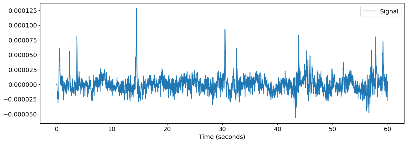
# Extract channel, convert to array, and average the channels
signal = raw.pick_channels(channels).get_data().mean(axis = 0)

nk.signal_plot(signal, sampling_rate=sampling_rate)

NOTE: pick_channels() is a legacy function. New code should use inst.pick(...).

Now, we can compute the complexity metrics of this signal.

Note that most complexity indices require some parameters to be specified, such as the delay or embedding dimension. We will used a dimension of 3 and a delay of 27 ms, that we need to convert into a number of samples (which depends on the sampling rate).

delay = int(27 / (1000 / sampling_rate))  # 27 is the delay in milliseconds

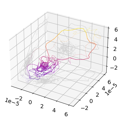
Let’s now compute the SVD Entropy of the signal. Importantly, note that there are a huge amount of possible indices to use (see what’s available in NeuroKit here).

# Note that for the example we cropped the signal to cut computation time
svden, info = nk.entropy_svd(signal[0:500], delay=delay, dimension=3, show=True)

print(f"SVDEn score: {svden:.2f}")

SVDEn score: 1.22

Event-related Complexity Analysis

Event-related Preprocessing (Epoching)

We will now create epochs around each event, and reject some based on extreme values.

epochs = mne.Epochs(raw, 
                    events, 
                    event_id=event_dict, 
                    tmin=-0.3, 
                    tmax=0.7, 
                    preload=True, 
                    verbose=False)

# Reject epochs by providing maximum peak-to-peak signal value thresholds
epochs = epochs.drop_bad(reject= dict(eeg=100e-6), verbose=False)  # 100 µV

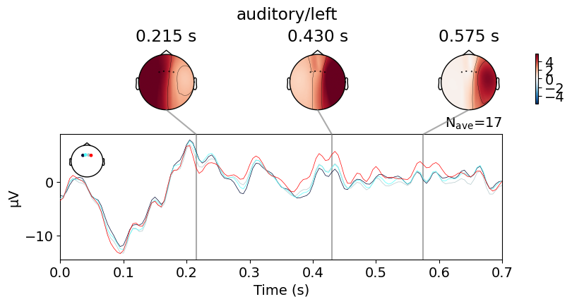
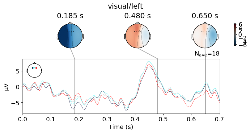
We can visualize the averaged events for each channel of interest as follows:

auditory = epochs['auditory/left'].pick_channels(channels).crop(tmin=0)
visual = epochs['visual/left'].pick_channels(channels).crop(tmin=0)

fig = auditory.average().plot_joint(title='auditory/left')
fig = visual.average().plot_joint(title='visual/left')

NOTE: pick_channels() is a legacy function. New code should use inst.pick(...).

NOTE: pick_channels() is a legacy function. New code should use inst.pick(...).

No projector specified for this dataset. Please consider the method self.add_proj.

No projector specified for this dataset. Please consider the method self.add_proj.

Now we are going to convert the data to a Pandas dataframe and concatenate the two groups of epochs. Next, we are going to average together the EEG channels.

df = pd.concat([auditory.to_data_frame(),
               visual.to_data_frame()])

df["EEG"] = df[channels].mean(axis=1)

df.head()

	time	condition	epoch	EEG 011	EEG 012	EEG 013	EEG 014	EEG
0	0.000	auditory/left	2	-4.414247	-3.515468	-0.330308	3.829678	-1.107586
1	0.005	auditory/left	2	-2.360910	-0.880196	1.669160	4.023423	0.612870
2	0.010	auditory/left	2	0.815137	2.031109	4.031405	6.675097	3.388187
3	0.015	auditory/left	2	1.605833	2.434812	4.953165	9.598465	4.648069
4	0.020	auditory/left	2	-0.559503	0.475777	3.917993	10.289093	3.530840

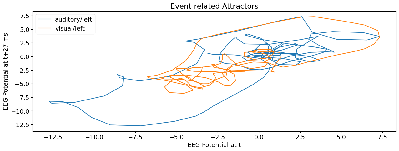
Event-related Attractors

Let’s visualize the attractors of the averaged events. We will then compute the complexity metrics for each epoch separately. We will re-use the delay parameters selected above, but this time with a dimension of 2 for easier visualization.

df_event = df.groupby(["time", "condition"], as_index=False).mean()

for cond in ["auditory/left", "visual/left"]:
    signal = df_event[df_event["condition"] == cond]["EEG"]
    attractor = nk.complexity_embedding(signal, delay=delay, dimension=2)
    plt.plot(attractor[:, 0], attractor[:, 1], label=cond)
plt.legend()
plt.xlabel("EEG Potential at t")
plt.ylabel("EEG Potential at t+27 ms")
plt.title("Event-related Attractors")

Text(0.5, 1.0, 'Event-related Attractors')

Compute complexity indices per epoch

def get_sdvden(x):
    rez, _ = nk.entropy_svd(x["EEG"], delay=delay, dimension=3)
    return pd.Series({'SVDEn': rez})

def get_hjorth(x):
    rez, _ = nk.entropy_svd(x["EEG"])
    return pd.Series({'Hjorth': rez})


results = pd.merge(
    df.groupby(["condition", "epoch"], as_index=False).apply(get_sdvden), 
    df.groupby(["condition", "epoch"], as_index=False).apply(get_hjorth)
)

results.head()

C:\Users\runneradmin\AppData\Local\Temp\ipykernel_4564\1026332364.py:11: DeprecationWarning: DataFrameGroupBy.apply operated on the grouping columns. This behavior is deprecated, and in a future version of pandas the grouping columns will be excluded from the operation. Either pass `include_groups=False` to exclude the groupings or explicitly select the grouping columns after groupby to silence this warning.
  df.groupby(["condition", "epoch"], as_index=False).apply(get_sdvden),
C:\Users\runneradmin\AppData\Local\Temp\ipykernel_4564\1026332364.py:12: DeprecationWarning: DataFrameGroupBy.apply operated on the grouping columns. This behavior is deprecated, and in a future version of pandas the grouping columns will be excluded from the operation. Either pass `include_groups=False` to exclude the groupings or explicitly select the grouping columns after groupby to silence this warning.
  df.groupby(["condition", "epoch"], as_index=False).apply(get_hjorth)

	condition	epoch	SVDEn	Hjorth
0	auditory/left	2	1.415754	0.576404
1	auditory/left	6	1.402700	0.484591
2	auditory/left	10	1.442964	0.614160
3	auditory/left	14	1.451905	0.588377
4	auditory/left	19	1.392537	0.535773

Lets’ run some t-tests on these indices.

scipy.stats.ttest_ind(results[results["condition"] == "auditory/left"]["SVDEn"], 
                      results[results["condition"] == "visual/left"]["SVDEn"], 
                      equal_var=False)

scipy.stats.ttest_ind(results[results["condition"] == "auditory/left"]["Hjorth"], 
                      results[results["condition"] == "visual/left"]["Hjorth"], 
                      equal_var=False)

TtestResult(statistic=0.3530201729161316, pvalue=0.7263454874826607, df=32.60499213593565)

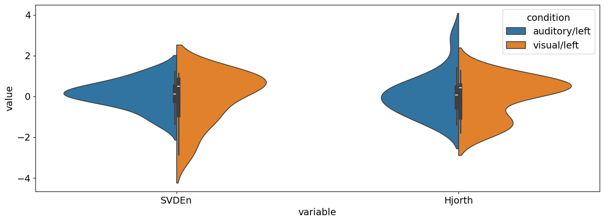
We can visualize these differences like follows:

# Standardize
results[['SVDEn', 'Hjorth']] = nk.standardize(results[['SVDEn', 'Hjorth']])

# Pivot to long format
results_long = pd.melt(results, id_vars=['condition', "epoch"], value_vars=['SVDEn', 'Hjorth'])

# Plot results
sns.violinplot(data=results_long, x="variable", y="value", hue="condition", split=True)

<Axes: xlabel='variable', ylabel='value'>

Fractal Density

Note: this index is totally exploratory and is mentioned here as part of a WIP development.

Now, we will average the signal of those 4 channels for each epoch and store them in a dictionary.