Benchmarking of ECG Preprocessing Methods

This study can be referenced by citing the package.

We’d like to publish this study, but unfortunately we currently don’t have the time. If you want to help to make it happen, please contact us!

Introduction

This work is a replication and extension of the work by Porr & Howell (2019), that compared the performance of different popular R-peak detectors.

Databases

Glasgow University Database

The GUDB Database (Howell & Porr, 2018) contains ECGs from 25 subjects. Each subject was recorded performing 5 different tasks for two minutes (sitting, doing a maths test on a tablet, walking on a treadmill, running on a treadmill, using a hand bike). The sampling rate is 250Hz for all the conditions.

The script to download and format the database using the ECG-GUDB Python package by Bernd Porr can be found here.

MIT-BIH Arrhythmia Database

The MIT-BIH Arrhythmia Database [MIT-Arrhythmia; Moody & Mark (2001)] contains 48 excerpts of 30-min of two-channel ambulatory ECG recordings sampled at 360Hz and 25 additional recordings from the same participants including common but clinically significant arrhythmias (denoted as the MIT-Arrhythmia-x database).

The script to download and format the database using the can be found here.

MIT-BIH Normal Sinus Rhythm Database

This database includes 18 clean long-term ECG recordings of subjects. Due to memory limits, we only kept the second hour of recording of each participant.

The script to download and format the database using the can be found here.

Lobachevsky University Electrocardiography Database

The Lobachevsky University Electrocardiography Database [LUDB; Kalyakulina et al. (2018)] consists of 200 10-second 12-lead ECG signal records representing different morphologies of the ECG signal. The ECGs were collected from healthy volunteers and patients, which had various cardiovascular diseases. The boundaries of P, T waves and QRS complexes were manually annotated by cardiologists for all 200 records.

Fantasia Database

The Fantasia database (Iyengar, Peng, Morin, Goldberger, & Lipsitz, 1996) consists of twenty young and twenty elderly healthy subjects. All subjects remained in a resting state in sinus rhythm while watching the movie Fantasia (Disney, 1940) to help maintain wakefulness. The continuous ECG signals were digitized at 250 Hz. Each heartbeat was annotated using an automated arrhythmia detection algorithm, and each beat annotation was verified by visual inspection.

Concanate them together

import pandas as pd

# Load ECGs
ecgs = ["../../data/gudb/ECGs.csv",
        "../../data/mit_arrhythmia/ECGs.csv",
        "../../data/mit_normal/ECGs.csv",
        "../../data/ludb/ECGs.csv",
        "../../data/fantasia/ECGs.csv"]

# Load True R-peaks location
rpeaks = [pd.read_csv("../../data/gudb/Rpeaks.csv"),
          pd.read_csv("../../data/mit_arrhythmia/Rpeaks.csv"),
          pd.read_csv("../../data/mit_normal/Rpeaks.csv"),
          pd.read_csv("../../data/ludb/Rpeaks.csv"),
          pd.read_csv("../../data/fantasia/Rpeaks.csv")]

Study 1: Comparing Different R-Peaks Detection Algorithms

Algorithm Comparison Procedure

Algorithm Comparison Setup Functions

import neurokit2 as nk

def neurokit(ecg, sampling_rate):
    signal, info = nk.ecg_peaks(ecg, sampling_rate=sampling_rate, method="neurokit")
    return info["ECG_R_Peaks"]

def pantompkins1985(ecg, sampling_rate):
    signal, info = nk.ecg_peaks(ecg, sampling_rate=sampling_rate, method="pantompkins1985")
    return info["ECG_R_Peaks"]

def hamilton2002(ecg, sampling_rate):
    signal, info = nk.ecg_peaks(ecg, sampling_rate=sampling_rate, method="hamilton2002")
    return info["ECG_R_Peaks"]

def martinez2003(ecg, sampling_rate):
    signal, info = nk.ecg_peaks(ecg, sampling_rate=sampling_rate, method="martinez2003")
    return info["ECG_R_Peaks"]

def christov2004(ecg, sampling_rate):
    signal, info = nk.ecg_peaks(ecg, sampling_rate=sampling_rate, method="christov2004")
    return info["ECG_R_Peaks"]

def gamboa2008(ecg, sampling_rate):
    signal, info = nk.ecg_peaks(ecg, sampling_rate=sampling_rate, method="gamboa2008")
    return info["ECG_R_Peaks"]

def elgendi2010(ecg, sampling_rate):
    signal, info = nk.ecg_peaks(ecg, sampling_rate=sampling_rate, method="elgendi2010")
    return info["ECG_R_Peaks"]

def engzeemod2012(ecg, sampling_rate):
    signal, info = nk.ecg_peaks(ecg, sampling_rate=sampling_rate, method="engzeemod2012")
    return info["ECG_R_Peaks"]

def kalidas2017(ecg, sampling_rate):
    signal, info = nk.ecg_peaks(ecg, sampling_rate=sampling_rate, method="kalidas2017")
    return info["ECG_R_Peaks"]

def rodrigues2020(ecg, sampling_rate):
    signal, info = nk.ecg_peaks(ecg, sampling_rate=sampling_rate, method="rodrigues2020")
    return info["ECG_R_Peaks"]

Run the Algorithm Comparison Benchmarks

Note: This takes a long time (several hours).

results = []
for method in [neurokit, pantompkins1985, hamilton2002, martinez2003, christov2004,
               gamboa2008, elgendi2010, engzeemod2012, kalidas2017, rodrigues2020]:
    for i in range(len(rpeaks)):
        data_ecg = pd.read_csv(ecgs[i])
        result = nk.benchmark_ecg_preprocessing(method, data_ecg, rpeaks[i])
        result["Method"] = method.__name__
        results.append(result)
results = pd.concat(results).reset_index(drop=True)

results.to_csv("data_detectors.csv", index=False)

Algorithm Comparison Results

library(tidyverse)
library(easystats)
library(lme4)

data <- read.csv("data_detectors.csv", stringsAsFactors = FALSE) %>%
  mutate(Method = fct_relevel(Method, "neurokit", "pantompkins1985", "hamilton2002", "martinez2003", "christov2004", "gamboa2008", "elgendi2010", "engzeemod2012", "kalidas2017", "rodrigues2020"))

colors <- c("neurokit"="#E91E63", "pantompkins1985"="#f44336", "hamilton2002"="#FF5722", "martinez2003"="#FF9800", "christov2004"="#FFC107", "gamboa2008"="#4CAF50", "elgendi2010"="#009688", "engzeemod2012"="#2196F3", "kalidas2017"="#3F51B5", "rodrigues2020"="#9C27B0")

Errors and bugs

data %>%
  mutate(Error = case_when(
    Error == "index -1 is out of bounds for axis 0 with size 0" ~ "index -1 out of bounds",
    Error == "index 0 is out of bounds for axis 0 with size 0" ~ "index 0 out of bounds",
    TRUE ~ Error)) %>%
  group_by(Database, Method) %>%
  mutate(n = n()) %>%
  group_by(Database, Method, Error) %>%
  summarise(Percentage = n() / unique(n)) %>%
  ungroup() %>%
  mutate(Error = fct_relevel(Error, "None")) %>%
  ggplot(aes(x=Error, y=Percentage, fill=Method)) +
    geom_bar(stat="identity", position = position_dodge2(preserve = "single")) +
    facet_wrap(~Database, nrow=5) +
    theme_modern() +
    theme(axis.text.x = element_text(size = 7, angle = 45, hjust = 1)) +
    scale_fill_manual(values=colors)

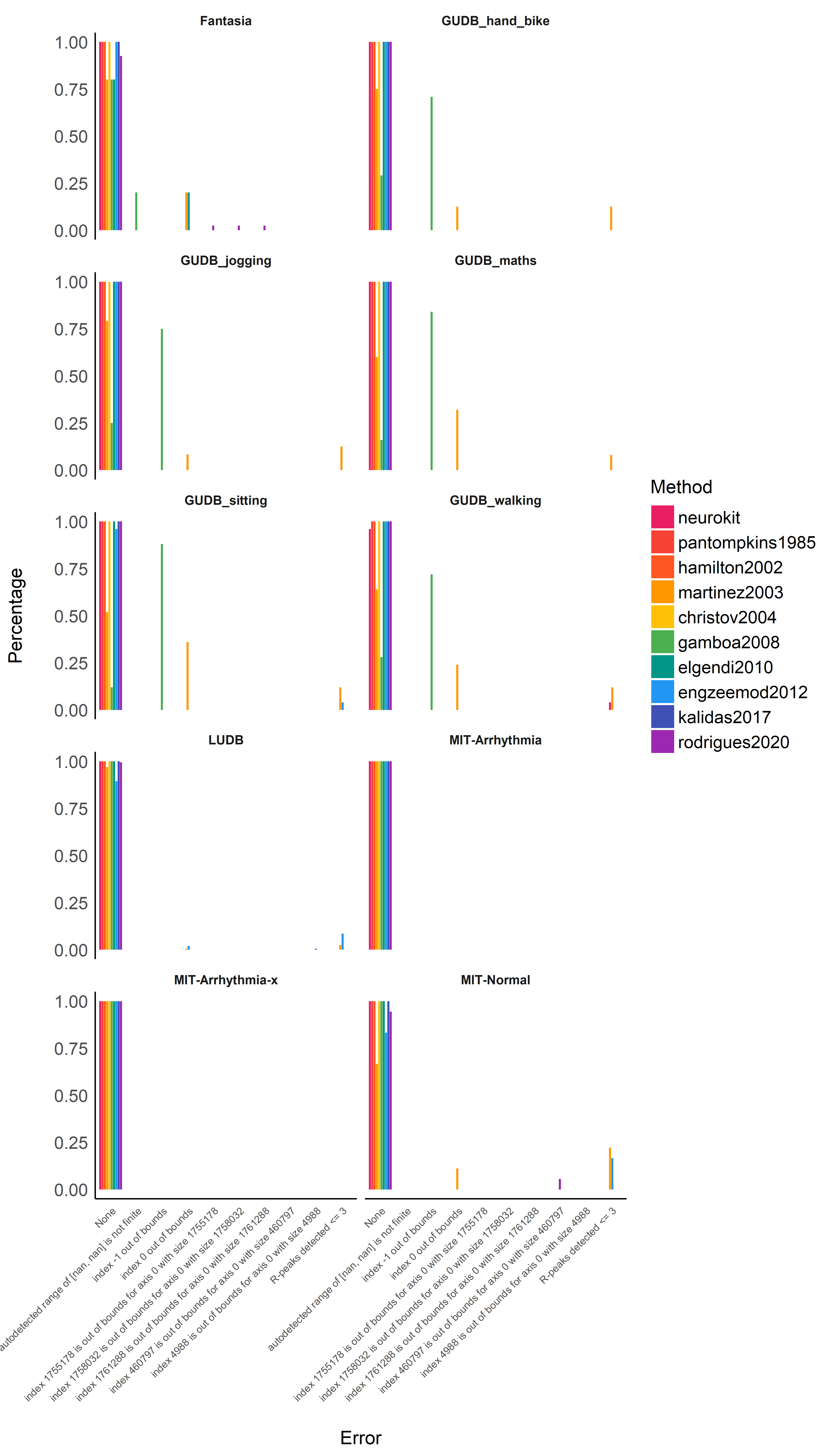
Conclusion: It seems that gamboa2008 and martinez2003 are particularly prone to errors, especially in the case of a noisy ECG signal. Aside from that, the other algorithms are quite resistant and bug-free.

data <- filter(data, Error == "None")
data <- filter(data, !is.na(Score))

Computation Time

Duration Descriptive Statistics

# Normalize duration
data <- data %>%
  mutate(Duration = (Duration) / (Recording_Length * Sampling_Rate))

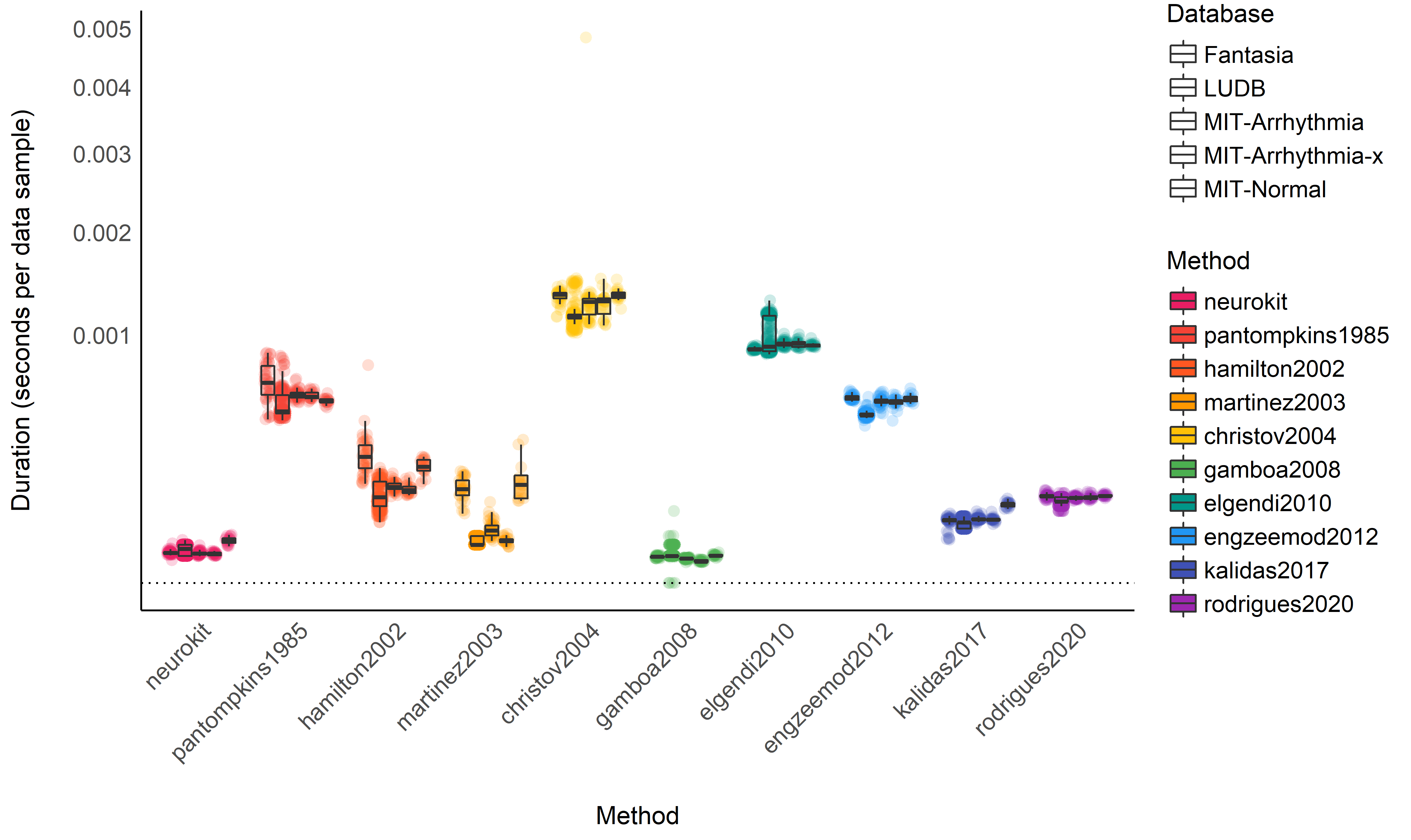
data %>%
  ggplot(aes(x=Method, y=Duration, fill=Method)) +
    geom_jitter2(aes(color=Method, group=Database), size=3, alpha=0.2, position=position_jitterdodge()) +
    geom_boxplot(aes(alpha=Database), outlier.alpha = 0) +
    geom_hline(yintercept=0, linetype="dotted") +
    theme_modern() +
    theme(axis.text.x = element_text(angle = 45, hjust = 1)) +
    scale_alpha_manual(values=seq(0, 1, length.out=8)) +
    scale_color_manual(values=colors) +
    scale_fill_manual(values=colors) +
    scale_y_sqrt() +
    ylab("Duration (seconds per data sample)")

Duration Statistical Modelling

model <- lmer(Duration ~ Method + (1|Database) + (1|Participant), data=data)

means <- modelbased::estimate_means(model)

arrange(means, Mean)
## Estimated Marginal Means
##
## Method          |     Mean |       SE |       95% CI
## ----------------------------------------------------
## gamboa2008      | 2.90e-05 | 1.18e-05 | [0.00, 0.00]
## neurokit        | 3.25e-05 | 1.17e-05 | [0.00, 0.00]
## martinez2003    | 6.59e-05 | 1.18e-05 | [0.00, 0.00]
## kalidas2017     | 7.80e-05 | 1.17e-05 | [0.00, 0.00]
## rodrigues2020   | 1.29e-04 | 1.17e-05 | [0.00, 0.00]
## hamilton2002    | 1.68e-04 | 1.17e-05 | [0.00, 0.00]
## engzeemod2012   | 5.10e-04 | 1.18e-05 | [0.00, 0.00]
## pantompkins1985 | 5.64e-04 | 1.17e-05 | [0.00, 0.00]
## elgendi2010     | 9.80e-04 | 1.18e-05 | [0.00, 0.00]
## christov2004    | 1.25e-03 | 1.17e-05 | [0.00, 0.00]
##
## Marginal means estimated at Method

means %>%
  ggplot(aes(x=Method, y=Mean, color=Method)) +
  geom_line(aes(group=1), size=1) +
  geom_pointrange(aes(ymin=CI_low, ymax=CI_high), size=1) +
  geom_hline(yintercept=0, linetype="dotted") +
  theme_modern() +
  theme(axis.text.x = element_text(angle = 45, hjust = 1)) +
  scale_color_manual(values=colors) +
    ylab("Duration (seconds per data sample)")

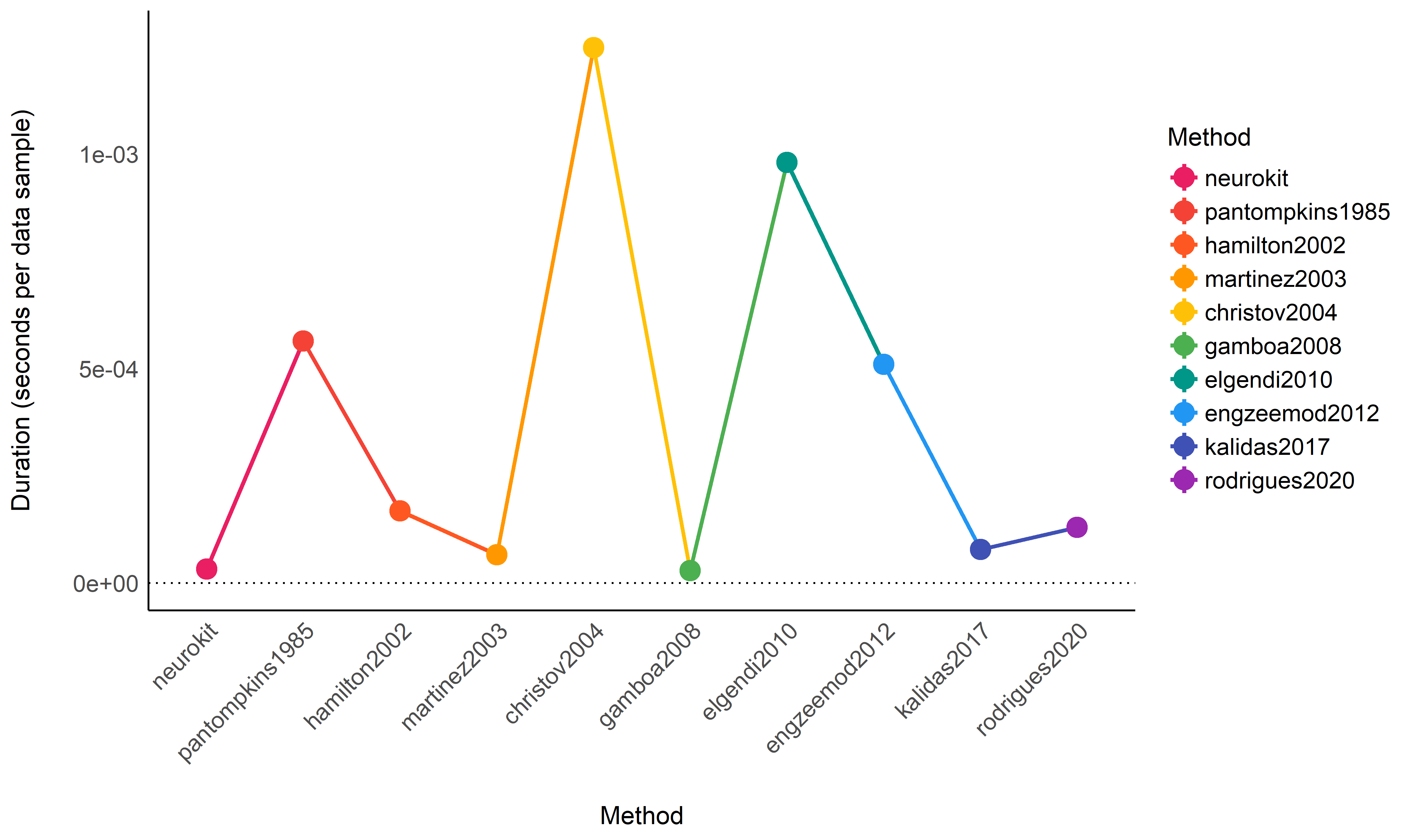
Conclusion: It seems that gamboa2008 and neurokit are the fastest methods, followed by martinez2003, kalidas2017, rodrigues2020 and hamilton2002. The other methods are then substantially slower.

Accuracy

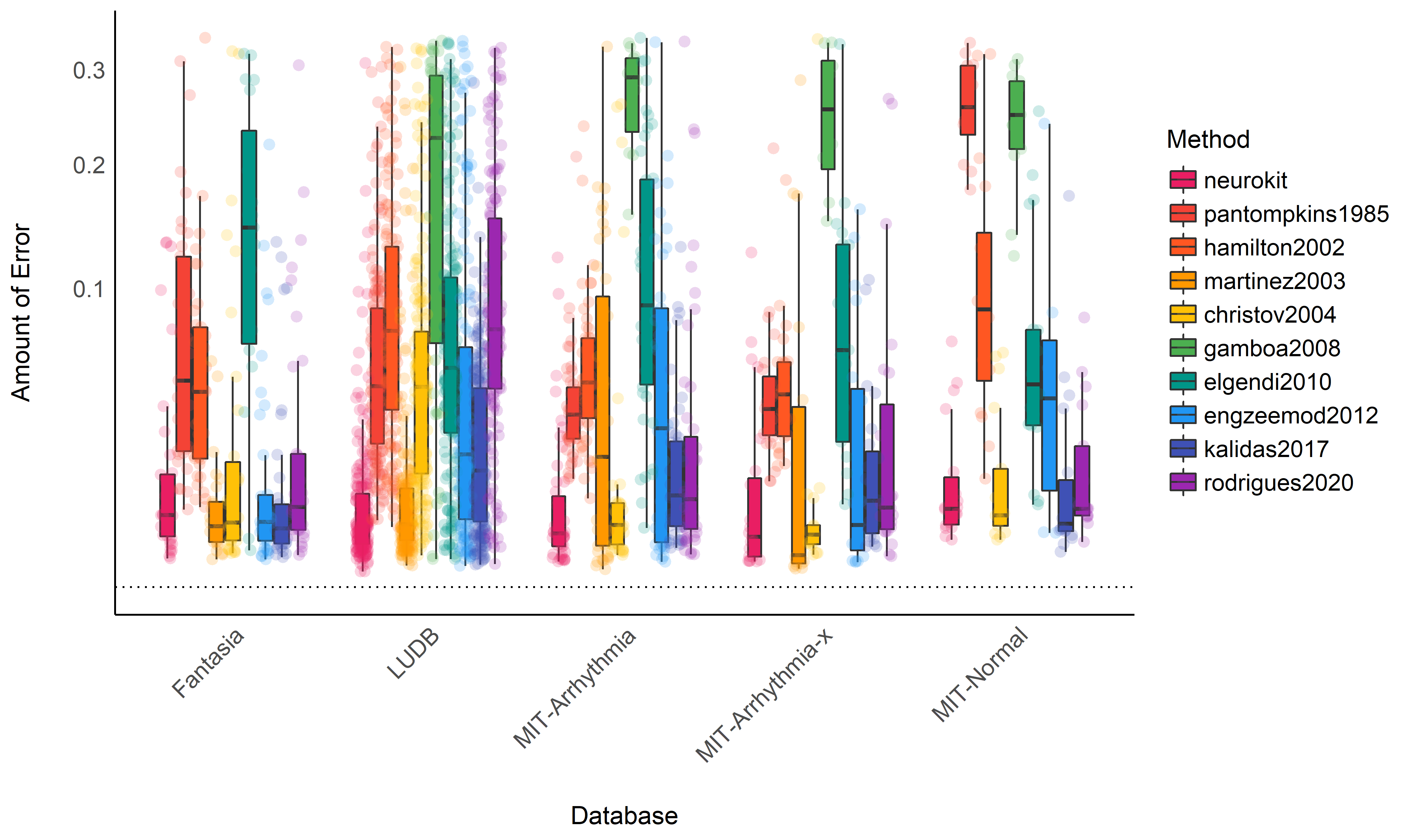
Note: The accuracy is computed as the absolute distance from the original “true” R-peaks location. As such, the closest to zero, the better the accuracy.

Performance Descriptive Statistics

data <- data %>%
  mutate(Outlier = performance::check_outliers(Score, threshold = list(zscore = stats::qnorm(p = 1 - 0.000001)))) %>%
  filter(Outlier == 0)

data %>%
  ggplot(aes(x=Database, y=Score)) +
    geom_boxplot(aes(fill=Method), outlier.alpha = 0, alpha=1) +
    geom_jitter2(aes(color=Method, group=Method), size=3, alpha=0.2, position=position_jitterdodge()) +
    geom_hline(yintercept=0, linetype="dotted") +
    theme_modern() +
    theme(axis.text.x = element_text(angle = 45, hjust = 1)) +
    scale_color_manual(values=colors) +
    scale_fill_manual(values=colors) +
    scale_y_sqrt() +
    ylab("Amount of Error")

Performance Statistical Modelling

model <- lmer(Score ~ Method + (1|Database) + (1|Participant), data=data)

means <- modelbased::estimate_means(model)

arrange(means, abs(Mean))
## Estimated Marginal Means
##
## Method          | Mean |       SE |       95% CI
## ------------------------------------------------
## neurokit        | 0.01 | 4.89e-03 | [0.00, 0.02]
## kalidas2017     | 0.02 | 4.90e-03 | [0.01, 0.03]
## martinez2003    | 0.02 | 5.25e-03 | [0.01, 0.03]
## christov2004    | 0.05 | 5.11e-03 | [0.04, 0.06]
## engzeemod2012   | 0.05 | 5.30e-03 | [0.04, 0.06]
## pantompkins1985 | 0.07 | 5.11e-03 | [0.06, 0.08]
## rodrigues2020   | 0.07 | 5.11e-03 | [0.06, 0.08]
## hamilton2002    | 0.08 | 5.18e-03 | [0.07, 0.09]
## elgendi2010     | 0.09 | 5.13e-03 | [0.08, 0.10]
## gamboa2008      | 0.22 | 8.02e-03 | [0.20, 0.24]
##
## Marginal means estimated at Method

means %>%
  ggplot(aes(x=Method, y=Mean, color=Method)) +
  geom_line(aes(group=1), size=1) +
  geom_pointrange(aes(ymin=CI_low, ymax=CI_high), size=1) +
  geom_hline(yintercept=0, linetype="dotted") +
  theme_modern() +
  theme(axis.text.x = element_text(angle = 45, hjust = 1)) +
  scale_color_manual(values=colors) +
    ylab("Amount of Error")

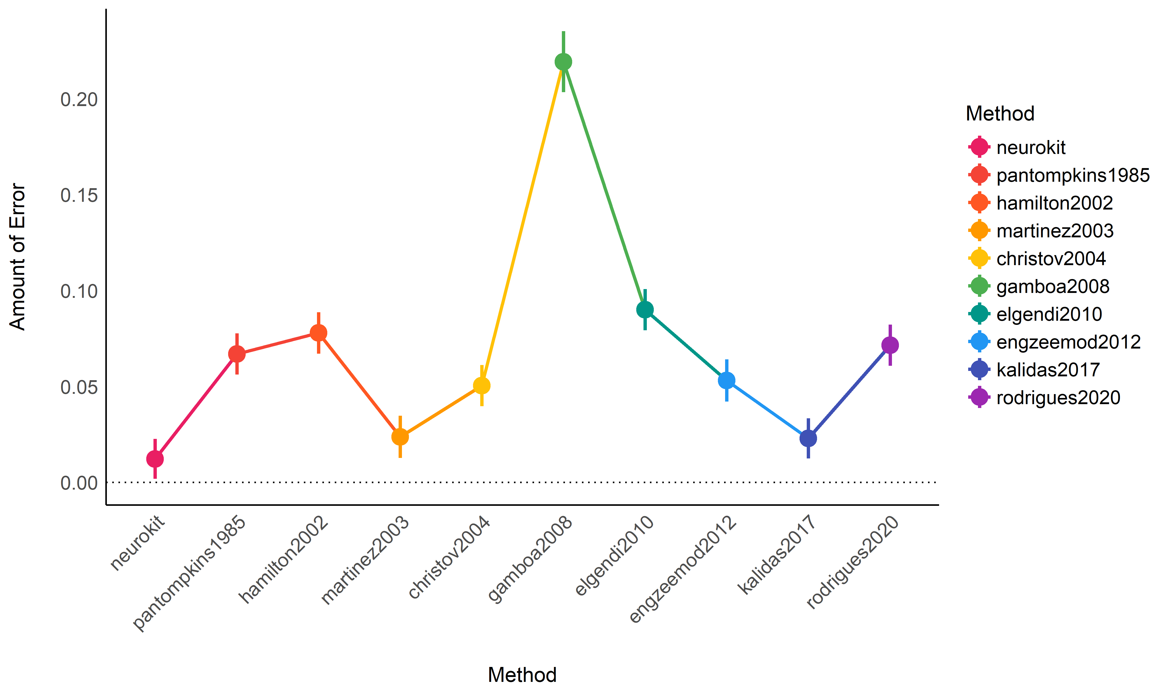
Conclusion: It seems that neurokit, kalidas2017 and martinez2003 the most accurate algorithms to detect R-peaks. This pattern of results differs a bit from Porr & Howell (2019) that outlines engzeemod2012, elgendi2010, kalidas2017 as the most accurate and christov2004, hamilton2002 and pantompkins1985 as the worse. Discrepancies could be due to the differences in data and analysis, as here we used more databases and modelled them by respecting their hierarchical structure using mixed models.

Algorithm Comparison Conclusion

Based on the accuracy / execution time criterion, it seems like neurokit is the best R-peak detection method, followed by kalidas2017.

Study 2: Normalization

Normalization Procedure

Normalization Setup Functions

import neurokit2 as nk

def none(ecg, sampling_rate):
    signal, info = nk.ecg_peaks(ecg, sampling_rate=sampling_rate, method="neurokit")
    return info["ECG_R_Peaks"]

def mean_detrend(ecg, sampling_rate):
    ecg = nk.signal_detrend(ecg, order=0)
    signal, info = nk.ecg_peaks(ecg, sampling_rate=sampling_rate, method="neurokit")
    return info["ECG_R_Peaks"]

def standardize(ecg, sampling_rate):
    ecg = nk.standardize(ecg)
    signal, info = nk.ecg_peaks(ecg, sampling_rate=sampling_rate, method="neurokit")
    return info["ECG_R_Peaks"]

Run the Normalization Benchmarks

Note: This takes a long time (several hours).

results = []
for method in [none, mean_detrend, standardize]:
    for i in range(len(rpeaks)):
        data_ecg = pd.read_csv(ecgs[i])
        result = nk.benchmark_ecg_preprocessing(method, data_ecg, rpeaks[i])
        result["Method"] = method.__name__
        results.append(result)
results = pd.concat(results).reset_index(drop=True)

results.to_csv("data_normalization.csv", index=False)

Normalization Results

library(tidyverse)
library(easystats)
library(lme4)

data <- read.csv("data_normalization.csv", stringsAsFactors = FALSE) %>%
  mutate(Database = ifelse(str_detect(Database, "GUDB"), paste0(str_replace(Database, "GUDB_", "GUDB ("), ")"), Database),
         Method = fct_relevel(Method, "none", "mean_removal", "standardization"),
         Participant = paste0(Database, Participant)) %>%
  filter(Error == "None") %>%
  filter(!is.na(Score))

colors <- c("none"="#607D8B", "mean_removal"="#673AB7", "standardization"="#00BCD4")

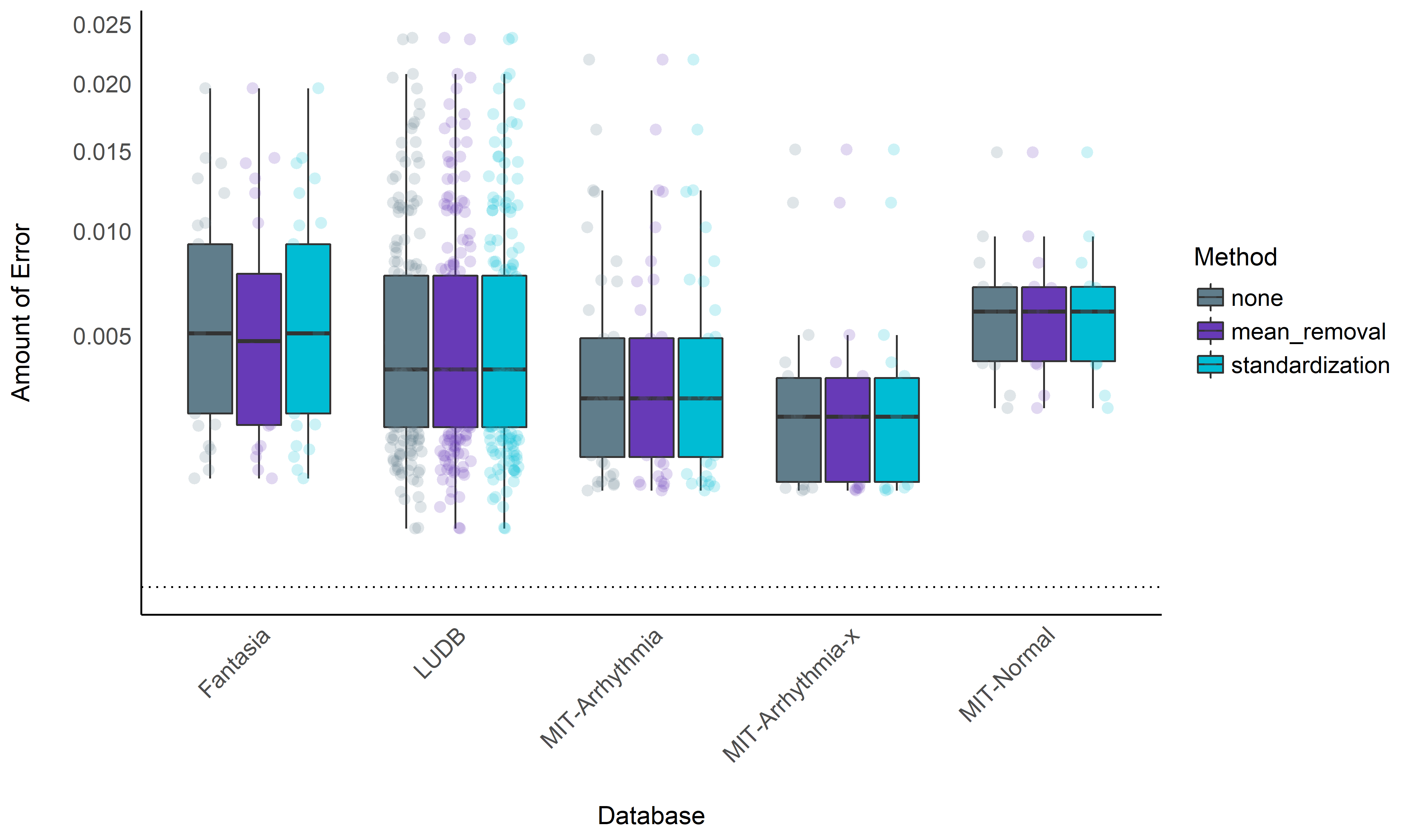
Normalized Accuracy

Normalized Performance Descriptive Statistics

data <- data %>%
  mutate(Outlier = performance::check_outliers(Score, threshold = list(zscore = stats::qnorm(p = 1 - 0.000001)))) %>%
  filter(Outlier == 0)

data %>%
  ggplot(aes(x=Database, y=Score)) +
    geom_boxplot(aes(fill=Method), outlier.alpha = 0, alpha=1) +
    geom_jitter2(aes(color=Method, group=Method), size=3, alpha=0.2, position=position_jitterdodge()) +
    geom_hline(yintercept=0, linetype="dotted") +
    theme_modern() +
    theme(axis.text.x = element_text(angle = 45, hjust = 1)) +
    scale_color_manual(values=colors) +
    scale_fill_manual(values=colors) +
    scale_y_sqrt() +
    ylab("Amount of Error")

Normalized Performance Statistical Modelling

model <- lmer(Score ~ Method + (1|Database) + (1|Participant), data=data)

modelbased::estimate_contrasts(model)
## Marginal Contrasts Analysis
##
## Level1       |          Level2 | Difference |        95% CI |       SE | t(553.00) |     p
## ------------------------------------------------------------------------------------------
## mean_removal | standardization |  -1.01e-07 | [ 0.00, 0.00] | 1.29e-07 |     -0.78 | 0.716
## none         |    mean_removal |  -8.72e-08 | [ 0.00, 0.00] | 1.29e-07 |     -0.68 | 0.777
## none         | standardization |  -1.88e-07 | [ 0.00, 0.00] | 1.28e-07 |     -1.47 | 0.308
##
## Marginal contrasts estimated at Method
## p-value adjustment method: Holm (1979)

means <- modelbased::estimate_means(model)
arrange(means, abs(Mean))
## Estimated Marginal Means
##
## Method          |     Mean |       SE |       95% CI
## ----------------------------------------------------
## none            | 5.23e-03 | 5.14e-04 | [0.00, 0.01]
## mean_removal    | 5.23e-03 | 5.14e-04 | [0.00, 0.01]
## standardization | 5.23e-03 | 5.14e-04 | [0.00, 0.01]
##
## Marginal means estimated at Method

means %>%
  ggplot(aes(x=Method, y=Mean, color=Method)) +
  geom_line(aes(group=1), size=1) +
  geom_pointrange(aes(ymin=CI_low, ymax=CI_high), size=1) +
  theme_modern() +
  theme(axis.text.x = element_text(angle = 45, hjust = 1)) +
  scale_color_manual(values=colors) +
    ylab("Amount of Error")

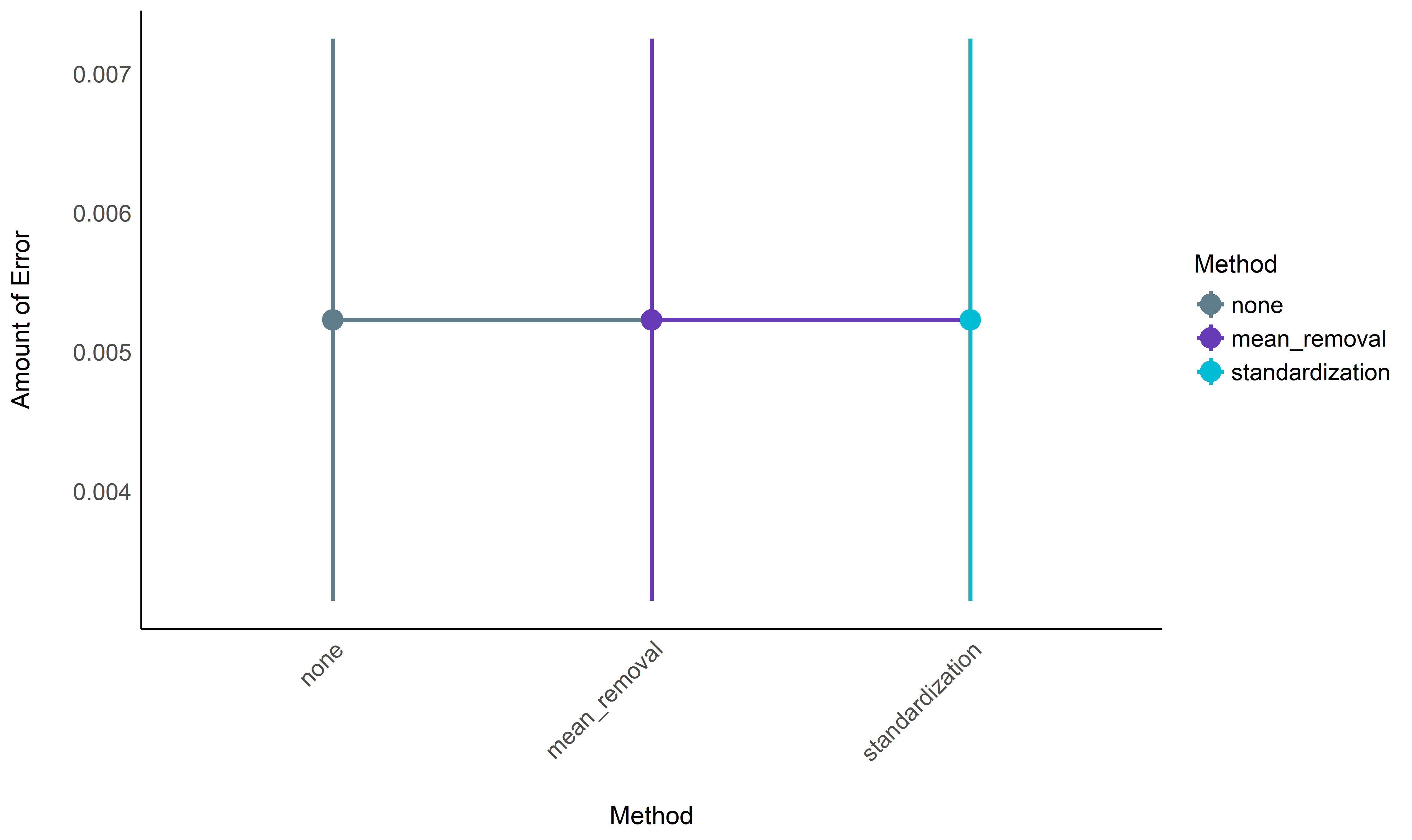
Normalization Conclusion

No significant benefits added by normalization for the neurokit method.

Study 3: Low Frequency Trends Removal

Trend Removal Procedure

Trend Removal Setup Functions

import neurokit2 as nk

def none(ecg, sampling_rate):
    signal, info = nk.ecg_peaks(ecg, sampling_rate=sampling_rate, method="neurokit")
    return info["ECG_R_Peaks"]

# Detrending-based
def polylength(ecg, sampling_rate):
    length = len(ecg) / sampling_rate
    ecg = nk.signal_detrend(ecg, method="polynomial", order=int(length / 2))
    signal, info = nk.ecg_peaks(ecg, sampling_rate=sampling_rate, method="neurokit")
    return info["ECG_R_Peaks"]

def tarvainen(ecg, sampling_rate):
    ecg = nk.signal_detrend(ecg, method="tarvainen2002")
    signal, info = nk.ecg_peaks(ecg, sampling_rate=sampling_rate, method="neurokit")
    return info["ECG_R_Peaks"]

def locreg(ecg, sampling_rate):
    ecg = nk.signal_detrend(ecg,
                            method="locreg",
                            window=1/0.5,
                            stepsize=0.02)
    signal, info = nk.ecg_peaks(ecg, sampling_rate=sampling_rate, method="neurokit")
    return info["ECG_R_Peaks"]

def rollingz(ecg, sampling_rate):
    ecg = nk.standardize(ecg, window=sampling_rate*2)
    signal, info = nk.ecg_peaks(ecg, sampling_rate=sampling_rate, method="neurokit")
    return info["ECG_R_Peaks"]

# Filtering-based

Run the Trend Removal Benchmarks

Note: This takes a very long time (several hours).

results = []
for method in [none, polylength, tarvainen, locreg, rollingz]:
    result = nk.benchmark_ecg_preprocessing(method, ecgs, rpeaks)
    result["Method"] = method.__name__
    results.append(result)
results = pd.concat(results).reset_index(drop=True)

results.to_csv("data_lowfreq.csv", index=False)

References

Howell, L., & Porr, B. (2018). High precision ECG database with annotated r peaks, recorded and filmed under realistic conditions.

Iyengar, N., Peng, C., Morin, R., Goldberger, A. L., & Lipsitz, L. A. (1996). Age-related alterations in the fractal scaling of cardiac interbeat interval dynamics. American Journal of Physiology-Regulatory, Integrative and Comparative Physiology, 271(4), R1078–R1084.

Kalyakulina, A. I., Yusipov, I. I., Moskalenko, V. A., Nikolskiy, A. V., Kozlov, A. A., Kosonogov, K. A., … Ivanchenko, M. V. (2018). LU electrocardiography database: A new open-access validation tool for delineation algorithms. arXiv Preprint arXiv:1809.03393.

Moody, G. B., & Mark, R. G. (2001). The impact of the MIT-BIH arrhythmia database. IEEE Engineering in Medicine and Biology Magazine, 20(3), 45–50.

Porr, B., & Howell, L. (2019). R-peak detector stress test with a new noisy ECG database reveals significant performance differences amongst popular detectors. bioRxiv, 722397.