Complexity, Fractals, and Entropy

Complexity, Fractals, and Entropy#

Main#

complexity()#

complexity(signal, which='makowski2022', delay=1, dimension=2, tolerance='sd', **kwargs)[source]#

Complexity and Chaos Analysis

Measuring the complexity of a signal refers to the quantification of various aspects related to concepts such as chaos, entropy, unpredictability, and fractal dimension.

Tip

We recommend checking our open-access review for an introduction to fractal physiology and its application in neuroscience.

There are many indices that have been developed and used to assess the complexity of signals, and all of them come with different specificities and limitations. While they should be used in an informed manner, it is also convenient to have a single function that can compute multiple indices at once.

The nk.complexity() function can be used to compute a useful subset of complexity metrics and features. While this is great for exploratory analyses, we recommend running each function separately, to gain more control over the parameters and information that you get.

Warning

The indices included in this function will be subjected to change in future versions, depending on what the literature suggests. We recommend using this function only for quick exploratory analyses, but then replacing it by the calls to the individual functions.

Check-out our open-access study explaining the selection of indices.

The categorization by “computation time” is based on our study results:

Parameters:

signal (Union[list, np.array, pd.Series]) – The signal (i.e., a time series) in the form of a vector of values.
which (list) – What metrics to compute. Can be “makowski2022”.
delay (int) – Time delay (often denoted Tau $\tau$, sometimes referred to as lag) in samples. See complexity_delay() to estimate the optimal value for this parameter.
dimension (int) – Embedding Dimension (m, sometimes referred to as d or order). See complexity_dimension() to estimate the optimal value for this parameter.
tolerance (float) – Tolerance (often denoted as r), distance to consider two data points as similar. If "sd" (default), will be set to $0.2 * SD_{signal}$. See complexity_tolerance() to estimate the optimal value for this parameter.

Returns:

df (pd.DataFrame) – A dataframe with one row containing the results for each metric as columns.
info (dict) – A dictionary containing additional information.

Examples

Example 1: Compute fast and medium-fast complexity metrics

In [1]: import neurokit2 as nk

# Simulate a signal of 3 seconds
In [2]: signal = nk.signal_simulate(duration=3, frequency=[5, 10])

# Compute selection of complexity metrics (Makowski et al., 2022)
In [3]: df, info = nk.complexity(signal, which = "makowski2022")

In [4]: df
Out[4]: 
      AttEn    BubbEn     CWPEn  ...  MFDFA_Width     MSPEn     SVDEn
0  0.519414  0.089258  0.000168  ...     0.905873  0.947385  0.164543

[1 rows x 15 columns]

Example 2: Compute complexity over time

In [5]: import numpy as np

In [6]: import pandas as pd

In [7]: import neurokit2 as nk

# Create dynamically varying noise
In [8]: amount_noise = nk.signal_simulate(duration=2, frequency=0.9)

In [9]: amount_noise = nk.rescale(amount_noise, [0, 0.5])

In [10]: noise = np.random.uniform(0, 2, len(amount_noise)) * amount_noise

# Add to simple signal
In [11]: signal = noise + nk.signal_simulate(duration=2, frequency=5)

In [12]: nk.signal_plot(signal, sampling_rate = 1000)

# Create function-wrappers that only return the index value
In [13]: pfd = lambda x: nk.fractal_petrosian(x)[0]

In [14]: kfd = lambda x: nk.fractal_katz(x)[0]

In [15]: sfd = lambda x: nk.fractal_sevcik(x)[0]

In [16]: svden = lambda x: nk.entropy_svd(x)[0]

In [17]: fisher = lambda x: -1 * nk.fisher_information(x)[0]  # FI is anticorrelated with complexity

# Use them in a rolling window
In [18]: rolling_kfd = pd.Series(signal).rolling(500, min_periods = 300, center=True).apply(kfd)

In [19]: rolling_pfd = pd.Series(signal).rolling(500, min_periods = 300, center=True).apply(pfd)

In [20]: rolling_sfd = pd.Series(signal).rolling(500, min_periods = 300, center=True).apply(sfd)

In [21]: rolling_svden = pd.Series(signal).rolling(500, min_periods = 300, center=True).apply(svden)

In [22]: rolling_fisher = pd.Series(signal).rolling(500, min_periods = 300, center=True).apply(fisher)

In [23]: nk.signal_plot([signal,
   ....:                 rolling_kfd.values,
   ....:                 rolling_pfd.values,
   ....:                 rolling_sfd.values,
   ....:                 rolling_svden.values,
   ....:                 rolling_fisher],
   ....:                 labels = ["Signal",
   ....:                          "Petrosian Fractal Dimension",
   ....:                          "Katz Fractal Dimension",
   ....:                          "Sevcik Fractal Dimension",
   ....:                          "SVD Entropy",
   ....:                          "Fisher Information"],
   ....:                sampling_rate = 1000,
   ....:                standardize = True)
   ....: 

References

Lau, Z. J., Pham, T., Chen, S. H. A., & Makowski, D. (2022). Brain entropy, fractal dimensions and predictability: A review of complexity measures for EEG in healthy and neuropsychiatric populations. European Journal of Neuroscience, 1-23.
Makowski, D., Te, A. S., Pham, T., Lau, Z. J., & Chen, S. H. (2022). The Structure of Chaos: An Empirical Comparison of Fractal Physiology Complexity Indices Using NeuroKit2. Entropy, 24 (8), 1036.

Parameters Choice#

complexity_delay()#

complexity_delay(signal, delay_max=50, method='fraser1986', algorithm=None, show=False, **kwargs)[source]#

Automated selection of the optimal Delay (Tau)

The time delay (Tau $\tau$, also referred to as Lag) is one of the two critical parameters (the other being the Dimension m) involved in the construction of the time-delay embedding of a signal. It corresponds to the delay in samples between the original signal and its delayed version(s). In other words, how many samples do we consider between a given state of the signal and its closest past state.

When $\tau$ is smaller than the optimal theoretical value, consecutive coordinates of the system’s state are correlated and the attractor is not sufficiently unfolded. Conversely, when $\tau$ is larger than it should be, successive coordinates are almost independent, resulting in an uncorrelated and unstructured cloud of points.

The selection of the parameters delay and *dimension* is a challenge. One approach is to select them (semi) independently (as dimension selection often requires the delay), using complexity_delay() and complexity_dimension(). However, some joint-estimation methods do exist, that attempt at finding the optimal delay and dimension at the same time.

Note also that some authors (e.g., Rosenstein, 1994) suggest identifying the optimal embedding dimension first, and that the optimal delay value should then be considered as the optimal delay between the first and last delay coordinates (in other words, the actual delay should be the optimal delay divided by the optimal embedding dimension minus 1).

Several authors suggested different methods to guide the choice of the delay:

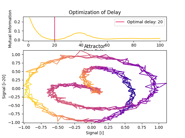
Fraser and Swinney (1986) suggest using the first local minimum of the mutual information between the delayed and non-delayed time series, effectively identifying a value of Tau for which they share the least information (and where the attractor is the least redundant). Unlike autocorrelation, mutual information takes into account also nonlinear correlations.
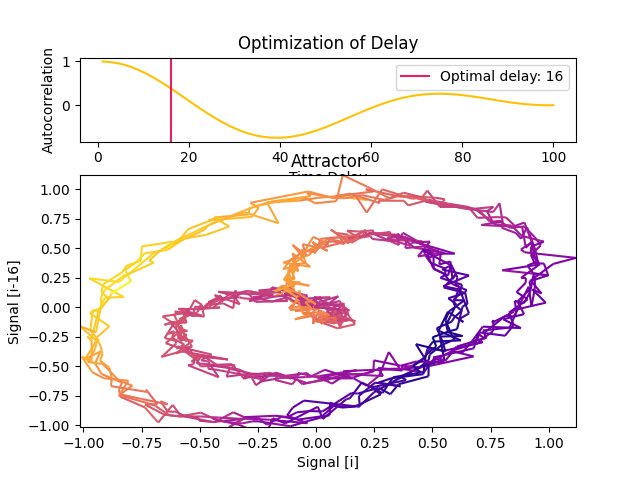
Theiler (1990) suggested to select Tau where the autocorrelation between the signal and its lagged version at Tau first crosses the value $1/e$. The autocorrelation-based methods have the advantage of short computation times when calculated via the fast Fourier transform (FFT) algorithm.
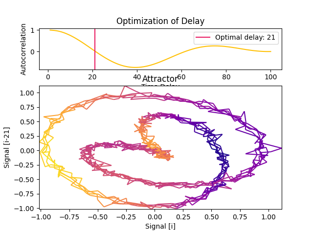
Casdagli (1991) suggests instead taking the first zero-crossing of the autocorrelation.
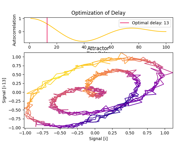
Rosenstein (1993) suggests to approximate the point where the autocorrelation function drops to $(1 - 1/e)$ of its maximum value.
Rosenstein (1994) suggests to the point close to 40% of the slope of the average displacement from the diagonal (ADFD).
Kim (1999) suggests estimating Tau using the correlation integral, called the C-C method, which has shown to agree with those obtained using the Mutual Information. This method makes use of a statistic within the reconstructed phase space, rather than analyzing the temporal evolution of the time series. However, computation times are significantly long for this method due to the need to compare every unique pair of pairwise vectors within the embedded signal per delay.
Lyle (2021) describes the “Symmetric Projection Attractor Reconstruction” (SPAR), where $1/3$ of the the dominant frequency (i.e., of the length of the average “cycle”) can be a suitable value for approximately periodic data, and makes the attractor sensitive to morphological changes. See also Aston’s talk. This method is also the fastest but might not be suitable for aperiodic signals. The algorithm argument (default to "fft") and will be passed as the method argument of signal_psd().

Joint-Methods for Delay and Dimension

Gautama (2003) mentions that in practice, it is common to have a fixed time lag and to adjust the embedding dimension accordingly. As this can lead to large m values (and thus to embedded data of a large size) and thus, slow processing, they describe an optimisation method to jointly determine m and $\tau$, based on the entropy ratio.

Note

We would like to implement the joint-estimation by Matilla-García et al. (2021), please get in touch if you can help us!

Parameters:

signal (Union[list, np.array, pd.Series]) – The signal (i.e., a time series) in the form of a vector of values.
delay_max (int) – The maximum time delay (Tau or lag) to test.
method (str) – The method that defines what to compute for each tested value of Tau. Can be one of "fraser1986", "theiler1990", "casdagli1991", "rosenstein1993", "rosenstein1994", "kim1999", or "lyle2021".
algorithm (str) – The method used to find the optimal value of Tau given the values computed by the method. If None (default), will select the algorithm according to the method. Modify only if you know what you are doing.
show (bool) – If True, will plot the metric values for each value of tau.
**kwargs (optional) – Additional arguments to be passed for C-C method.

Returns:

delay (int) – Optimal time delay.
parameters (dict) – A dictionary containing additional information regarding the parameters used to compute optimal time-delay embedding.

Examples

Example 1: Comparison of different methods for estimating the optimal delay of an simple artificial signal.

In [1]: import neurokit2 as nk

In [2]: signal = nk.signal_simulate(duration=10, sampling_rate=100, frequency=[1, 1.5], noise=0.02)

In [3]: nk.signal_plot(signal)

In [4]: delay, parameters = nk.complexity_delay(signal, delay_max=100, show=True,
   ...:                                         method="fraser1986")
   ...: 

In [5]: delay, parameters = nk.complexity_delay(signal, delay_max=100, show=True,
   ...:                                         method="theiler1990")
   ...: 

In [6]: delay, parameters = nk.complexity_delay(signal, delay_max=100, show=True,
   ...:                                         method="casdagli1991")
   ...: 

In [7]: delay, parameters = nk.complexity_delay(signal, delay_max=100, show=True,
   ...:                                         method="rosenstein1993")
   ...: 

In [8]: delay, parameters = nk.complexity_delay(signal, delay_max=100, show=True,
   ...:                                         method="rosenstein1994")
   ...: 

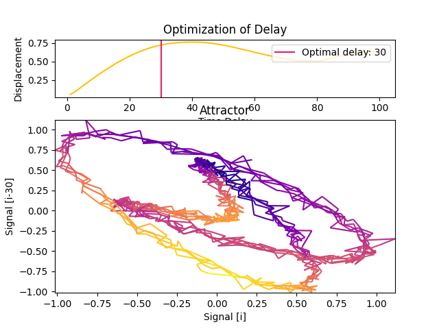
In [9]: delay, parameters = nk.complexity_delay(signal, delay_max=100, show=True,
   ...:                                         method="lyle2021")
   ...: 

Example 2: Optimizing the delay and the dimension using joint-estimation methods.

In [10]: delay, parameters = nk.complexity_delay(
   ....:     signal,
   ....:     delay_max=np.arange(1, 30, 1),  # Can be an int or a list
   ....:     dimension_max=20,  # Can be an int or a list
   ....:     method="gautama2003",
   ....:     surrogate_n=5,  # Number of surrogate signals to generate
   ....:     surrogate_method="random",  # can be IAAFT, see nk.signal_surrogate()
   ....:     show=True)
   ....: 

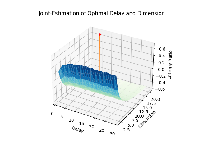
# Optimal dimension
In [11]: dimension = parameters["Dimension"]

In [12]: dimension
Out[12]: 20

Note: A double-checking of that method would be appreciated! Please help us improve.

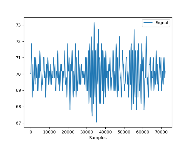
Example 3: Using a realistic signal.

In [13]: ecg = nk.ecg_simulate(duration=60*6, sampling_rate=200)

In [14]: signal = nk.ecg_rate(nk.ecg_peaks(ecg, sampling_rate=200),
   ....:                      sampling_rate=200,
   ....:                      desired_length=len(ecg))
   ....: 

In [15]: nk.signal_plot(signal)

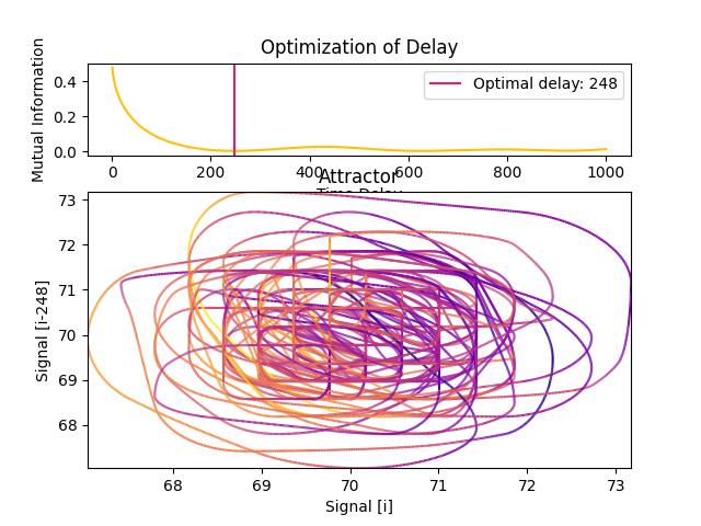
In [16]: delay, parameters = nk.complexity_delay(signal, delay_max=1000, show=True)

References

Lyle, J. V., Nandi, M., & Aston, P. J. (2021). Symmetric Projection Attractor Reconstruction: Sex Differences in the ECG. Frontiers in cardiovascular medicine, 1034.
Gautama, T., Mandic, D. P., & Van Hulle, M. M. (2003, April). A differential entropy based method for determining the optimal embedding parameters of a signal. In 2003 IEEE International Conference on Acoustics, Speech, and Signal Processing, 2003. Proceedings. (ICASSP’03). (Vol. 6, pp. VI-29). IEEE.
Camplani, M., & Cannas, B. (2009). The role of the embedding dimension and time delay in time series forecasting. IFAC Proceedings Volumes, 42(7), 316-320.
Rosenstein, M. T., Collins, J. J., & De Luca, C. J. (1993). A practical method for calculating largest Lyapunov exponents from small data sets. Physica D: Nonlinear Phenomena, 65(1-2), 117-134.
Rosenstein, M. T., Collins, J. J., & De Luca, C. J. (1994). Reconstruction expansion as a geometry-based framework for choosing proper delay times. Physica-Section D, 73(1), 82-98.
Kim, H., Eykholt, R., & Salas, J. D. (1999). Nonlinear dynamics, delay times, and embedding windows. Physica D: Nonlinear Phenomena, 127(1-2), 48-60.
Gautama, T., Mandic, D. P., & Van Hulle, M. M. (2003, April). A differential entropy based method for determining the optimal embedding parameters of a signal. In 2003 IEEE International Conference on Acoustics, Speech, and Signal Processing, 2003. Proceedings. (ICASSP’03). (Vol. 6, pp. VI-29). IEEE.
Camplani, M., & Cannas, B. (2009). The role of the embedding dimension and time delay in time series forecasting. IFAC Proceedings Volumes, 42(7), 316-320.

complexity_dimension()#

complexity_dimension(signal, delay=1, dimension_max=20, method='afnn', show=False, **kwargs)[source]#

Automated selection of the optimal Embedding Dimension (m)

The Embedding Dimension (m, sometimes referred to as d or order) is the second critical parameter (the first being the delay $\tau$) involved in the construction of the time-delay embedding of a signal. It corresponds to the number of delayed states (versions of the signals lagged by $\tau$) that we include in the embedding.

Though one can commonly find values of 2 or 3 used in practice, several authors suggested different numerical methods to guide the choice of m:

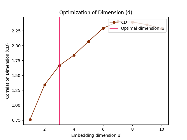
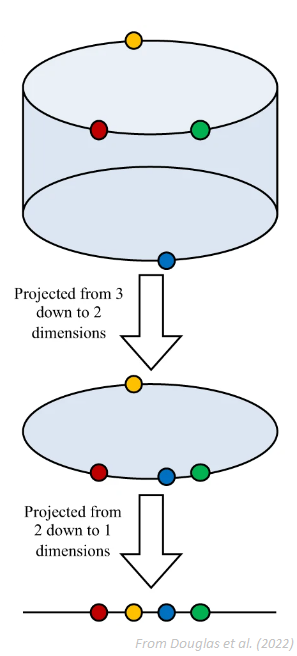
Correlation Dimension (CD): One of the earliest method to estimate the optimal m was to calculate the correlation dimension for embeddings of various sizes and look for a saturation (i.e., a plateau) in its value as the embedding dimension increases. One of the limitation is that a saturation will also occur when there is not enough data to adequately fill the high-dimensional space (note that, in general, having such large embeddings that it significantly shortens the length of the signal is not recommended).
FNN (False Nearest Neighbour): The method, introduced by Kennel et al. (1992), is based on the assumption that two points that are near to each other in the sufficient embedding dimension should remain close as the dimension increases. The algorithm checks the neighbours in increasing embedding dimensions until it finds only a negligible number of false neighbours when going from dimension $m$ to $m+1$. This corresponds to the lowest embedding dimension, which is presumed to give an unfolded space-state reconstruction. This method can fail in noisy signals due to the futile attempt of unfolding the noise (and in purely random signals, the amount of false neighbors does not substantially drops as m increases). The figure below show how projections to higher-dimensional spaces can be used to detect false nearest neighbours. For instance, the red and the yellow points are neighbours in the 1D space, but not in the 2D space.

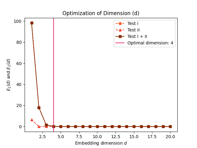
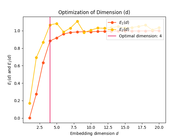
Illustration of FNN (Douglas et al., 2022).

AFN (Average False Neighbors): This modification by Cao (1997) of the FNN method addresses one of its main drawback, the need for a heuristic choice for the tolerance thresholds r. It uses the maximal Euclidian distance to represent nearest neighbors, and averages all ratios of the distance in $m+1$ to $m$ dimension and defines E1 and E2 as parameters. The optimal dimension corresponds to when E1 stops changing (reaches a plateau). E1 reaches a plateau at a dimension d0 if the signal comes from an attractor. Then d0*+1 is the optimal minimum embedding dimension. *E2 is a useful quantity to distinguish deterministic signals from stochastic signals. A constant E2 close to 1 for any embedding dimension d suggests random data, since the future values are independent of the past values.

Parameters:

signal (Union[list, np.array, pd.Series]) – The signal (i.e., a time series) in the form of a vector of values.
delay (int) – Time delay (often denoted Tau $\tau$, sometimes referred to as Lag) in samples. See complexity_delay() to choose the optimal value for this parameter.
dimension_max (int) – The maximum embedding dimension to test.
method (str) – Can be "afn" (Average False Neighbor), "fnn" (False Nearest Neighbour), or "cd" (Correlation Dimension).
show (bool) – Visualize the result.
**kwargs – Other arguments, such as R=10.0 or A=2.0 (relative and absolute tolerance, only for 'fnn' method).

Returns:

dimension (int) – Optimal embedding dimension.
parameters (dict) – A dictionary containing additional information regarding the parameters used to compute the optimal dimension.

Examples

In [1]: import neurokit2 as nk

In [2]: signal = nk.signal_simulate(duration=2, frequency=[5, 7, 8], noise=0.01)

# Correlation Dimension
In [3]: optimal_dimension, info = nk.complexity_dimension(signal,
   ...:                                                   delay=20,
   ...:                                                   dimension_max=10,
   ...:                                                   method='cd',
   ...:                                                   show=True)
   ...: 

# FNN
In [4]: optimal_dimension, info = nk.complexity_dimension(signal,
   ...:                                                   delay=20,
   ...:                                                   dimension_max=20,
   ...:                                                   method='fnn',
   ...:                                                   show=True)
   ...: 

# AFNN
In [5]: optimal_dimension, info = nk.complexity_dimension(signal,
   ...:                                                   delay=20,
   ...:                                                   dimension_max=20,
   ...:                                                   method='afnn',
   ...:                                                   show=True)
   ...: 

References

Kennel, M. B., Brown, R., & Abarbanel, H. D. (1992). Determining embedding dimension for phase-space reconstruction using a geometrical construction. Physical review A, 45(6), 3403.
Cao, L. (1997). Practical method for determining the minimum embedding dimension of a scalar time series. Physica D: Nonlinear Phenomena, 110(1-2), 43-50.
Rhodes, C., & Morari, M. (1997). The false nearest neighbors algorithm: An overview. Computers & Chemical Engineering, 21, S1149-S1154.
Krakovská, A., Mezeiová, K., & Budáčová, H. (2015). Use of false nearest neighbours for selecting variables and embedding parameters for state space reconstruction. Journal of Complex Systems, 2015.
Gautama, T., Mandic, D. P., & Van Hulle, M. M. (2003, April). A differential entropy based method for determining the optimal embedding parameters of a signal. In 2003 IEEE International Conference on Acoustics, Speech, and Signal Processing, 2003. Proceedings. (ICASSP’03). (Vol. 6, pp. VI-29). IEEE.

complexity_tolerance()#

complexity_tolerance(signal, method='maxApEn', r_range=None, delay=None, dimension=None, show=False)[source]#

Automated selection of tolerance (r)

Estimate and select the optimal tolerance (r) parameter used by other entropy and other complexity algorithms.

Many complexity algorithms are built on the notion of self-similarity and recurrence, and how often a system revisits its past states. Considering two states as identical is straightforward for discrete systems (e.g., a sequence of "A", "B" and "C" states), but for continuous signals, we cannot simply look for when the two numbers are exactly the same. Instead, we have to pick a threshold by which to consider two points as similar.

The tolerance r is essentially this threshold value (the numerical difference between two similar points that we “tolerate”). This parameter has a critical impact and is a major source of inconsistencies in the literature.

Different methods have been described to estimate the most appropriate tolerance value:

maxApEn: Different values of tolerance will be tested and the one where the approximate entropy (ApEn) is maximized will be selected and returned (Chen, 2008).
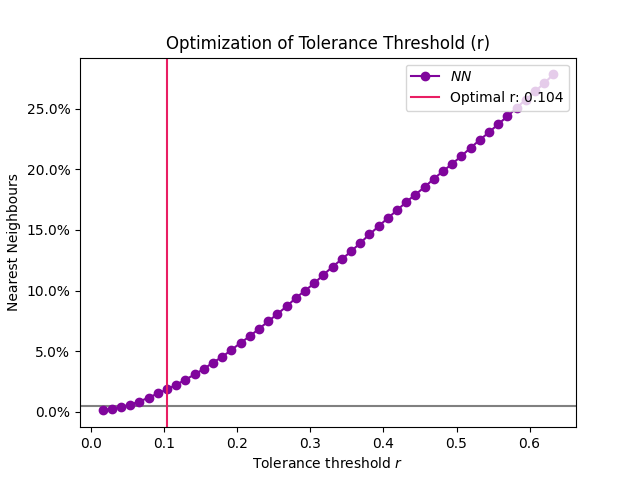
recurrence: The tolerance that yields a recurrence rate (see RQA) close to 1% will be returned. Note that this method is currently not suited for very long signals, as it is based on a recurrence matrix, which size is close to n^2. Help is needed to address this limitation.
neighbours: The tolerance that yields a number of nearest neighbours (NN) close to 2% will be returned.

As these methods are computationally expensive, other fast heuristics are available:

sd: r = 0.2 * standard deviation (SD) of the signal will be returned. This is the most commonly used value in the literature, though its appropriateness is questionable.
makowski: Adjusted value based on the SD, the embedding dimension and the signal’s length. See our study.
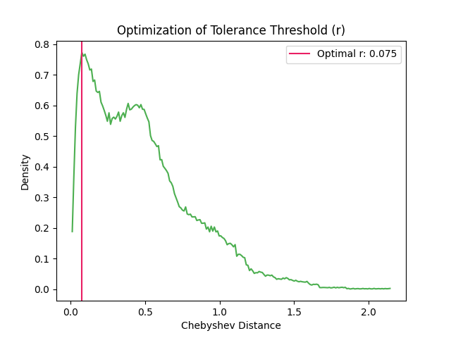
nolds: Adjusted value based on the SD and the dimension. The rationale is that the chebyshev distance (used in various metrics) rises logarithmically with increasing dimension. 0.5627 * np.log(dimension) + 1.3334 is the logarithmic trend line for the chebyshev distance of vectors sampled from a univariate normal distribution. A constant of 0.1164 is used so that tolerance = 0.2 * SDs for dimension = 2 (originally in CSchoel/nolds).
singh2016: Makes a histogram of the Chebyshev distance matrix and returns the upper bound of the modal bin.
chon2009: Acknowledging that computing multiple ApEns is computationally expensive, Chon (2009) suggested an approximation based a heuristic algorithm that takes into account the length of the signal, its short-term and long-term variability, and the embedding dimension m. Initially defined only for m in [2-7], we expanded this to work with value of m (though the accuracy is not guaranteed beyond m = 4).

Parameters:

signal (Union[list, np.array, pd.Series]) – The signal (i.e., a time series) in the form of a vector of values.
method (str) – Can be "maxApEn" (default), "sd", "recurrence", "neighbours", "nolds", "chon2009", or "neurokit".
r_range (Union[list, int]) – The range of tolerance values (or the number of values) to test. Only used if method is "maxApEn" or "recurrence". If None (default), the default range will be used; np.linspace(0.02, 0.8, r_range) * np.std(signal, ddof=1) for "maxApEn", and np. linspace(0, np.max(d), 30 + 1)[1:] for "recurrence". You can set a lower number for faster results.
delay (int) – Only used if method="maxApEn". See entropy_approximate().
dimension (int) – Only used if method="maxApEn". See entropy_approximate().
show (bool) – If True and method is "maxApEn", will plot the ApEn values for each value of r.

Returns:

float – The optimal tolerance value.
dict – A dictionary containing additional information.

Examples

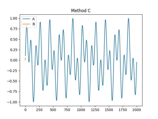
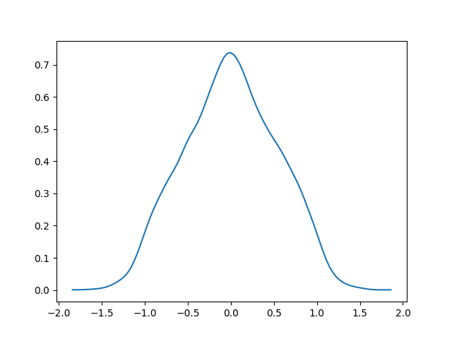
Example 1: The method based on the SD of the signal is fast. The plot shows the d distribution of the values making the signal, and the width of the arrow represents the chosen r parameter.

In [1]: import neurokit2 as nk

# Simulate signal
In [2]: signal = nk.signal_simulate(duration=2, frequency=[5, 7, 9, 12, 15])

# Fast method (based on the standard deviation)
In [3]: r, info = nk.complexity_tolerance(signal, method = "sd", show=True)

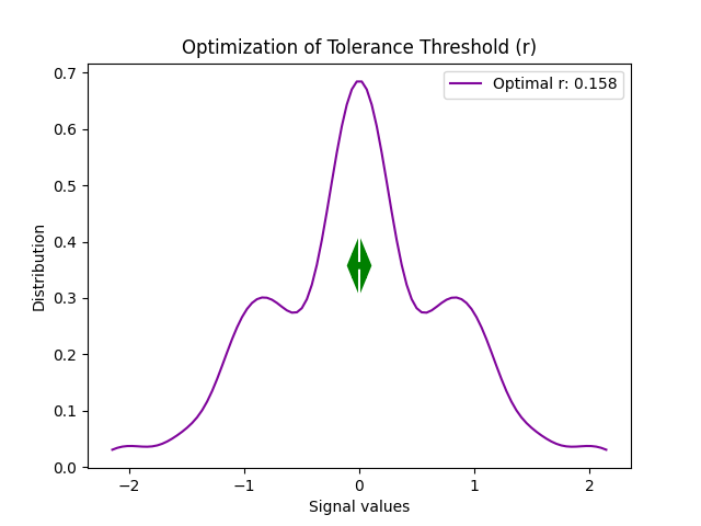
In [4]: r
Out[4]: 0.1581534263085267

The dimension can be taken into account: .. ipython:: python

# nolds method @savefig p_complexity_tolerance2.png scale=100% r, info = nk.complexity_tolerance(signal, method = “nolds”, dimension=3, show=True) @suppress plt.close()

In [5]: r
Out[5]: 0.1581534263085267

Example 2: The method based on the recurrence rate will display the rates according to different values of tolerance. The horizontal line indicates 5%.

In [6]: r, info = nk.complexity_tolerance(signal, delay=1, dimension=10,
   ...:                                   method = 'recurrence', show=True)
   ...: 

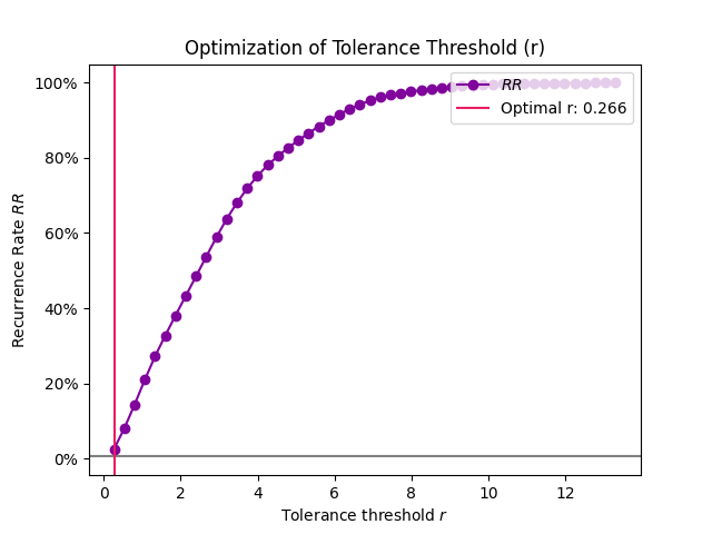
In [7]: r
Out[7]: 0.2662934154435781

An alternative, better suited for long signals is to use nearest neighbours.

In [8]: r, info = nk.complexity_tolerance(signal, delay=1, dimension=10,
   ...:                                   method = 'neighbours', show=True)
   ...: 

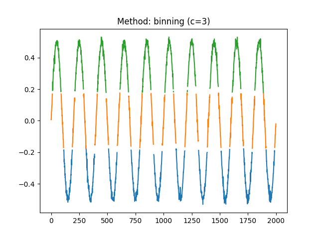
Another option is to use the density of distances.

In [9]: r, info = nk.complexity_tolerance(signal, delay=1, dimension=3,
   ...:                                   method = 'bin', show=True)
   ...: 

Example 3: The default method selects the tolerance at which ApEn is maximized.

# Slow method
In [10]: r, info = nk.complexity_tolerance(signal, delay=8, dimension=6,
   ....:                                   method = 'maxApEn', show=True)
   ....: 

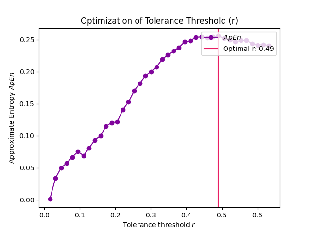
In [11]: r
Out[11]: 0.4902756215564327

Example 4: The tolerance values that are tested can be modified to get a more precise estimate.

# Narrower range
In [12]: r, info = nk.complexity_tolerance(signal, delay=8, dimension=6, method = 'maxApEn',
   ....:                                   r_range=np.linspace(0.002, 0.8, 30), show=True)
   ....: 

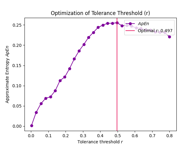
In [13]: r
Out[13]: 0.4973103448275862

References

Chon, K. H., Scully, C. G., & Lu, S. (2009). Approximate entropy for all signals. IEEE engineering in medicine and biology magazine, 28(6), 18-23.
Lu, S., Chen, X., Kanters, J. K., Solomon, I. C., & Chon, K. H. (2008). Automatic selection of the threshold value r for approximate entropy. IEEE Transactions on Biomedical Engineering, 55(8), 1966-1972.
Chen, X., Solomon, I. C., & Chon, K. H. (2008). Parameter selection criteria in approximate entropy and sample entropy with application to neural respiratory signals. Am. J. Physiol. Regul. Integr. Comp. Physiol.
Singh, A., Saini, B. S., & Singh, D. (2016). An alternative approach to approximate entropy threshold value (r) selection: application to heart rate variability and systolic blood pressure variability under postural challenge. Medical & biological engineering & computing, 54(5), 723-732.

complexity_k()#

complexity_k(signal, k_max='max', show=False)[source]#

Automated selection of k for Higuchi Fractal Dimension (HFD)

The optimal k-max is computed based on the point at which HFD values plateau for a range of k-max values (see Vega, 2015).

Parameters:

signal (Union[list, np.array, pd.Series]) – The signal (i.e., a time series) in the form of a vector of values.
k_max (Union[int, str, list], optional) – Maximum number of interval times (should be greater than or equal to 3) to be tested. If max, it selects the maximum possible value corresponding to half the length of the signal.
show (bool) – Visualise the slope of the curve for the selected kmax value.

Returns:

k (float) – The optimal kmax of the time series.
info (dict) – A dictionary containing additional information regarding the parameters used to compute optimal kmax.

See also

fractal_higuchi

Examples

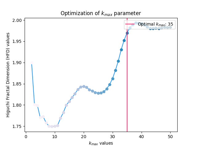
In [1]: import neurokit2 as nk

In [2]: signal = nk.signal_simulate(duration=2, sampling_rate=100, frequency=[5, 6], noise=0.5)

In [3]: k_max, info = nk.complexity_k(signal, k_max='default', show=True)

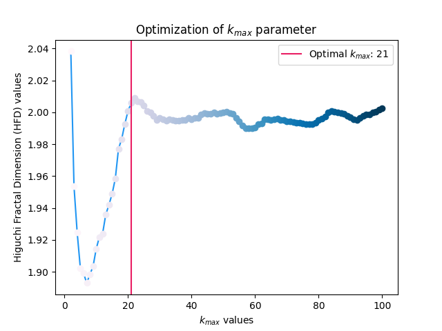
In [4]: k_max
Out[4]: 19

References

Higuchi, T. (1988). Approach to an irregular time series on the basis of the fractal theory. Physica D: Nonlinear Phenomena, 31(2), 277-283.
Vega, C. F., & Noel, J. (2015, June). Parameters analyzed of Higuchi’s fractal dimension for EEG brain signals. In 2015 Signal Processing Symposium (SPSympo) (pp. 1-5). IEEE. https:// ieeexplore.ieee.org/document/7168285

Fractal Dimension#

fractal_katz()#

fractal_katz(signal)[source]#

Katz’s Fractal Dimension (KFD)

Computes Katz’s Fractal Dimension (KFD). The euclidean distances between successive points in the signal are summed and averaged, and the maximum distance between the starting point and any other point in the sample.

Fractal dimensions range from 1.0 for straight lines, through approximately 1.15 for random-walks, to approaching 1.5 for the most convoluted waveforms.

Parameters:

signal (Union[list, np.array, pd.Series]) – The signal (i.e., a time series) in the form of a vector of values.

Returns:

kfd (float) – Katz’s fractal dimension of the single time series.
info (dict) – A dictionary containing additional information (currently empty, but returned nonetheless for consistency with other functions).

See also

fractal_linelength

Examples

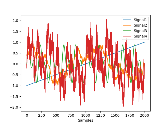
Step 1. Simulate different kinds of signals

In [1]: import neurokit2 as nk

In [2]: import numpy as np

# Simulate straight line
In [3]: straight = np.linspace(-1, 1, 2000)

# Simulate random
In [4]: random = nk.complexity_simulate(duration=2, method="randomwalk")

In [5]: random = nk.rescale(random, [-1, 1])

# Simulate simple
In [6]: simple = nk.signal_simulate(duration=2, frequency=[5, 10])

# Simulate complex
In [7]: complex = nk.signal_simulate(duration=2,
   ...:                              frequency=[1, 3, 6, 12],
   ...:                              noise = 0.1)
   ...: 

In [8]: nk.signal_plot([straight, random, simple, complex])

Step 2. Compute KFD for each of them

In [9]: KFD, _ = nk.fractal_katz(straight)

In [10]: KFD
Out[10]: 1.0

In [11]: KFD, _ = nk.fractal_katz(random)

In [12]: KFD
Out[12]: 1.9019643810898508

In [13]: KFD, _ = nk.fractal_katz(simple)

In [14]: KFD
Out[14]: 2.041857476392026

In [15]: KFD, _ = nk.fractal_katz(complex)

In [16]: KFD
Out[16]: 4.065032485461998

References

Katz, M. J. (1988). Fractals and the analysis of waveforms. Computers in Biology and Medicine, 18(3), 145-156. doi:10.1016/0010-4825(88)90041-8.

fractal_linelength()#

fractal_linelength(signal)[source]#

Line Length (LL)

Line Length (LL, also known as curve length), stems from a modification of the Katz fractal dimension algorithm, with the goal of making it more efficient and accurate (especially for seizure onset detection).

It basically corresponds to the average of the absolute consecutive differences of the signal, and was made to be used within subwindows. Note that this does not technically measure the fractal dimension, but the function was named with the fractal_ prefix due to its conceptual similarity with Katz’s fractal dimension.

Parameters:

signal (Union[list, np.array, pd.Series]) – The signal (i.e., a time series) in the form of a vector of values.

Returns:

float – Line Length.
dict – A dictionary containing additional information (currently empty, but returned nonetheless for consistency with other functions).

See also

fractal_katz

Examples

In [1]: import neurokit2 as nk

In [2]: signal = nk.signal_simulate(duration=2, sampling_rate=200, frequency=[5, 6, 10])

In [3]: ll, _ = nk.fractal_linelength(signal)

In [4]: ll
Out[4]: 0.11575342908508135

References

Esteller, R., Echauz, J., Tcheng, T., Litt, B., & Pless, B. (2001, October). Line length: an efficient feature for seizure onset detection. In 2001 Conference Proceedings of the 23rd Annual International Conference of the IEEE Engineering in Medicine and Biology Society (Vol. 2, pp. 1707-1710). IEEE.

fractal_petrosian()#

fractal_petrosian(signal, symbolize='C', show=False)[source]#

Petrosian fractal dimension (PFD)

Petrosian (1995) proposed a fast method to estimate the fractal dimension by converting the signal into a binary sequence from which the fractal dimension is estimated. Several variations of the algorithm exist (e.g., "A", "B", "C" or "D"), primarily differing in the way the discrete (symbolic) sequence is created (see func:complexity_symbolize for details). The most common method ("C", by default) binarizes the signal by the sign of consecutive differences.

\[\frac{log(N)}{log(N) + log(\frac{N}{N+0.4N_{\delta}})}\]

Most of these methods assume that the signal is periodic (without a linear trend). Linear detrending might be useful to eliminate linear trends (see signal_detrend()).

See also

information_mutual, entropy_svd

Parameters:

signal (Union[list, np.array, pd.Series]) – The signal (i.e., a time series) in the form of a vector of values.
symbolize (str) – Method to convert a continuous signal input into a symbolic (discrete) signal. By default, assigns 0 and 1 to values below and above the mean. Can be None to skip the process (in case the input is already discrete). See complexity_symbolize() for details.
show (bool) – If True, will show the discrete the signal.

Returns:

pfd (float) – The petrosian fractal dimension (PFD).
info (dict) – A dictionary containing additional information regarding the parameters used to compute PFD.

Examples

In [1]: import neurokit2 as nk

In [2]: signal = nk.signal_simulate(duration=2, frequency=[5, 12])

In [3]: pfd, info = nk.fractal_petrosian(signal, symbolize = "C", show=True)

$savefig/p_fractal_petrosian1.png$

In [4]: pfd
Out[4]: 1.0012592763505226

In [5]: info
Out[5]: {'Symbolization': 'C'}

References

Esteller, R., Vachtsevanos, G., Echauz, J., & Litt, B. (2001). A comparison of waveform fractal dimension algorithms. IEEE Transactions on Circuits and Systems I: Fundamental Theory and Applications, 48(2), 177-183.
Petrosian, A. (1995, June). Kolmogorov complexity of finite sequences and recognition of different preictal EEG patterns. In Proceedings eighth IEEE symposium on computer-based medical systems (pp. 212-217). IEEE.
Kumar, D. K., Arjunan, S. P., & Aliahmad, B. (2017). Fractals: applications in biological Signalling and image processing. CRC Press.
Goh, C., Hamadicharef, B., Henderson, G., & Ifeachor, E. (2005, June). Comparison of fractal dimension algorithms for the computation of EEG biomarkers for dementia. In 2nd International Conference on Computational Intelligence in Medicine and Healthcare (CIMED2005).

fractal_sevcik()#

fractal_sevcik(signal)[source]#

Sevcik Fractal Dimension (SFD)

The SFD algorithm was proposed to calculate the fractal dimension of waveforms by Sevcik (1998). This method can be used to quickly measure the complexity and randomness of a signal.

Note

Some papers (e.g., Wang et al. 2017) suggest adding np.log(2) to the numerator, but it’s unclear why, so we sticked to the original formula for now. But if you have an idea, please let us know!

Parameters:

signal (Union[list, np.array, pd.Series]) – The signal (i.e., a time series) in the form of a vector of values.

Returns:

sfd (float) – The sevcik fractal dimension.
info (dict) – An empty dictionary returned for consistency with the other complexity functions.

See also

fractal_petrosian

Examples

In [1]: import neurokit2 as nk

In [2]: signal = nk.signal_simulate(duration=2, frequency=5)

In [3]: sfd, _ = nk.fractal_sevcik(signal)

In [4]: sfd
Out[4]: 1.361438527611129

References

Sevcik, C. (2010). A procedure to estimate the fractal dimension of waveforms. arXiv preprint arXiv:1003.5266.
Kumar, D. K., Arjunan, S. P., & Aliahmad, B. (2017). Fractals: applications in biological Signalling and image processing. CRC Press.
Wang, H., Li, J., Guo, L., Dou, Z., Lin, Y., & Zhou, R. (2017). Fractal complexity-based feature extraction algorithm of communication signals. Fractals, 25(04), 1740008.
Goh, C., Hamadicharef, B., Henderson, G., & Ifeachor, E. (2005, June). Comparison of fractal dimension algorithms for the computation of EEG biomarkers for dementia. In 2nd International Conference on Computational Intelligence in Medicine and Healthcare (CIMED2005).

fractal_nld()#

fractal_nld(signal, corrected=False)[source]#

Fractal dimension via Normalized Length Density (NLDFD)

NLDFD is a very simple index corresponding to the average absolute consecutive differences of the (standardized) signal (np.mean(np.abs(np.diff(std_signal)))). This method was developed for measuring signal complexity of very short durations (< 30 samples), and can be used for instance when continuous signal FD changes (or “running” FD) are of interest (by computing it on sliding windows, see example).

For methods such as Higuchi’s FD, the standard deviation of the window FD increases sharply when the epoch becomes shorter. The NLD method results in lower standard deviation especially for shorter epochs, though at the expense of lower accuracy in average window FD.

See also

fractal_higuchi

Parameters:

signal (Union[list, np.array, pd.Series]) – The signal (i.e., a time series) in the form of a vector of values.
corrected (bool) – If True, will rescale the output value according to the power model estimated by Kalauzi et al. (2009) to make it more comparable with “true” FD range, as follows: FD = 1.9079*((NLD-0.097178)^0.18383). Note that this can result in np.nan if the result of the difference is negative.

Returns:

fd (DataFrame) – A dataframe containing the fractal dimension across epochs.
info (dict) – A dictionary containing additional information (currently, but returned nonetheless for consistency with other functions).

Examples

Example 1: Usage on a short signal

In [1]: import neurokit2 as nk

# Simulate a short signal with duration of 0.5s
In [2]: signal = nk.signal_simulate(duration=0.5, frequency=[3, 5])

# Compute Fractal Dimension
In [3]: fd, _ = nk.fractal_nld(signal, corrected=False)

In [4]: fd
Out[4]: 0.023124767861850155

Example 2: Compute FD-NLD on non-overlapping windows

In [5]: import numpy as np

# Simulate a long signal with duration of 5s
In [6]: signal = nk.signal_simulate(duration=5, frequency=[3, 5, 10], noise=0.1)

# We want windows of size=100 (0.1s)
In [7]: n_windows = len(signal) // 100  # How many windows

# Split signal into windows
In [8]: windows = np.array_split(signal, n_windows)

# Compute FD-NLD on all windows
In [9]: nld = [nk.fractal_nld(i, corrected=False)[0] for i in windows]

In [10]: np.mean(nld)  # Get average
Out[10]: 0.5988549518761661

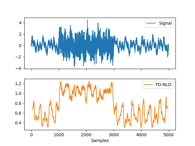
Example 3: Calculate FD-NLD on sliding windows

# Simulate a long signal with duration of 5s
In [11]: signal = nk.signal_simulate(duration=5, frequency=[3, 5, 10], noise=0.1)

# Add period of noise
In [12]: signal[1000:3000] = signal[1000:3000] + np.random.normal(0, 1, size=2000)

# Create function-wrapper that only return the NLD value
In [13]: nld = lambda x: nk.fractal_nld(x, corrected=False)[0]

# Use them in a rolling window of 100 samples (0.1s)
In [14]: rolling_nld = pd.Series(signal).rolling(100, min_periods = 100, center=True).apply(nld)

In [15]: nk.signal_plot([signal, rolling_nld], subplots=True, labels=["Signal", "FD-NLD"])

References

Kalauzi, A., Bojić, T., & Rakić, L. (2009). Extracting complexity waveforms from one-dimensional signals. Nonlinear biomedical physics, 3(1), 1-11.

fractal_psdslope()#

fractal_psdslope(signal, method='voss1988', show=False, **kwargs)[source]#

Fractal dimension via Power Spectral Density (PSD) slope

Fractal exponent can be computed from Power Spectral Density slope (PSDslope) analysis in signals characterized by a frequency power-law dependence.

It first transforms the time series into the frequency domain, and breaks down the signal into sine and cosine waves of a particular amplitude that together “add-up” to represent the original signal. If there is a systematic relationship between the frequencies in the signal and the power of those frequencies, this will reveal itself in log-log coordinates as a linear relationship. The slope of the best fitting line is taken as an estimate of the fractal scaling exponent and can be converted to an estimate of the fractal dimension.

A slope of 0 is consistent with white noise, and a slope of less than 0 but greater than -1, is consistent with pink noise i.e., 1/f noise. Spectral slopes as steep as -2 indicate fractional Brownian motion, the epitome of random walk processes.

Parameters:

signal (Union[list, np.array, pd.Series]) – The signal (i.e., a time series) in the form of a vector of values.
method (str) – Method to estimate the fractal dimension from the slope, can be "voss1988" (default) or "hasselman2013".
show (bool) – If True, returns the log-log plot of PSD versus frequency.
**kwargs – Other arguments to be passed to signal_psd() (such as method).

Returns:

slope (float) – Estimate of the fractal dimension obtained from PSD slope analysis.
info (dict) – A dictionary containing additional information regarding the parameters used to perform PSD slope analysis.

Examples

In [1]: import neurokit2 as nk

# Simulate a Signal with Laplace Noise
In [2]: signal = nk.signal_simulate(duration=2, sampling_rate=200, frequency=[5, 6], noise=0.5)

# Compute the Fractal Dimension from PSD slope
In [3]: psdslope, info = nk.fractal_psdslope(signal, show=True)

$savefig/p_fractal_psdslope1.png$

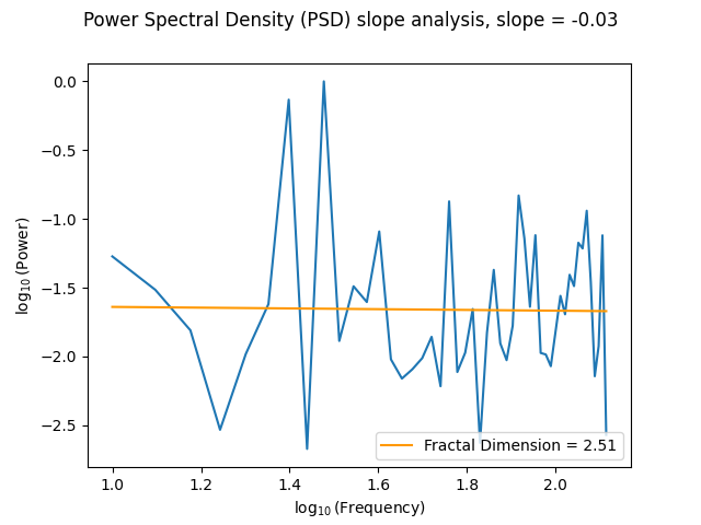
In [4]: psdslope
Out[4]: 2.531853434949906

References

https://complexity-methods.github.io/book/power-spectral-density-psd-slope.html
Hasselman, F. (2013). When the blind curve is finite: dimension estimation and model inference based on empirical waveforms. Frontiers in Physiology, 4, 75. https://doi.org/10.3389/fphys.2013.00075
Voss, R. F. (1988). Fractals in nature: From characterization to simulation. The Science of Fractal Images, 21-70.
Eke, A., Hermán, P., Kocsis, L., and Kozak, L. R. (2002). Fractal characterization of complexity in temporal physiological signals. Physiol. Meas. 23, 1-38.

fractal_higuchi()#

fractal_higuchi(signal, k_max='default', show=False, **kwargs)[source]#

Higuchi’s Fractal Dimension (HFD)

The Higuchi’s Fractal Dimension (HFD) is an approximate value for the box-counting dimension for time series. It is computed by reconstructing k-max number of new data sets. For each reconstructed data set, curve length is computed and plotted against its corresponding k-value on a log-log scale. HFD corresponds to the slope of the least-squares linear trend.

Values should fall between 1 and 2. For more information about the k parameter selection, see the complexity_k() optimization function.

Parameters:

signal (Union[list, np.array, pd.Series]) – The signal (i.e., a time series) in the form of a vector of values.
k_max (str or int) – Maximum number of interval times (should be greater than or equal to 2). If "default", the optimal k-max is estimated using complexity_k(), which is slow.
show (bool) – Visualise the slope of the curve for the selected k_max value.
**kwargs (optional) – Currently not used.

Returns:

HFD (float) – Higuchi’s fractal dimension of the time series.
info (dict) – A dictionary containing additional information regarding the parameters used to compute Higuchi’s fractal dimension.

See also

complexity_k

Examples

In [1]: import neurokit2 as nk

In [2]: signal = nk.signal_simulate(duration=1, sampling_rate=100, frequency=[3, 6], noise = 0.2)

In [3]: k_max, info =  nk.complexity_k(signal, k_max='default', show=True)

In [4]: hfd, info = nk.fractal_higuchi(signal, k_max=k_max, show=True)

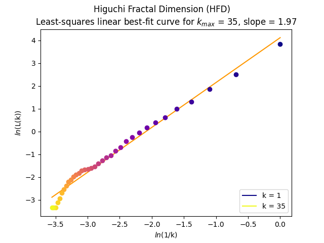
$savefig/p_fractal_higuchi1.png$ $savefig/p_fractal_higuchi2.png$

In [5]: hfd
Out[5]: 1.964685476951274

References

Higuchi, T. (1988). Approach to an irregular time series on the basis of the fractal theory. Physica D: Nonlinear Phenomena, 31(2), 277-283.
Vega, C. F., & Noel, J. (2015, June). Parameters analyzed of Higuchi’s fractal dimension for EEG brain signals. In 2015 Signal Processing Symposium (SPSympo) (pp. 1-5). IEEE. https://ieeexplore.ieee.org/document/7168285

fractal_density()#

fractal_density(signal, delay=1, tolerance='sd', bins=None, show=False, **kwargs)[source]#

Density Fractal Dimension (DFD)

This is a Work in Progress (WIP). The idea is to find a way of, essentially, averaging attractors. Because one can not directly average the trajectories, one way is to convert the attractor to a 2D density matrix that we can use similarly to a time-frequency heatmap. However, it is very unclear how to then derive meaningful indices from this density plot. Also, how many bins, or smoothing, should one use?

Basically, this index is exploratory and should not be used in its state. However, if you’re interested in the problem of “average” attractors (e.g., from multiple epochs / trials), and you want to think about it with us, feel free to let us know!

Parameters:

signal (Union[list, np.array, pd.Series]) – The signal (i.e., a time series) in the form of a vector of values.
delay (int) – Time delay (often denoted Tau $\tau$, sometimes referred to as lag) in samples. See complexity_delay() to estimate the optimal value for this parameter.
tolerance (float) – Tolerance (often denoted as r), distance to consider two data points as similar. If "sd" (default), will be set to $0.2 * SD_{signal}$. See complexity_tolerance() to estimate the optimal value for this parameter.
bins (int) – If not None but an integer, will use this value for the number of bins instead of a value based on the tolerance parameter.
show (bool) – Plot the density matrix. Defaults to False.
**kwargs – Other arguments to be passe.

Returns:

dfd (float) – The density fractal dimension.
info (dict) – A dictionary containing additional information.

Examples

In [1]: import neurokit2 as nk

In [2]: signal = nk.signal_simulate(duration=2, frequency=[5, 9], noise=0.01)

In [3]: dfd, _ = nk.fractal_density(signal, delay=20, show=True)

$savefig/p_fractal_density1.png$

In [4]: signal = nk.signal_simulate(duration=4, frequency=[5, 10, 11], noise=0.01)

In [5]: epochs = nk.epochs_create(signal, events=20)

In [6]: dfd, info1 = nk.fractal_density(epochs, delay=20, bins=20, show=True)

$savefig/p_fractal_density2.png$

Compare the complexity of two signals.

Warning

Help is needed to find a way to make statistics and comparing two density maps.

In [7]: import matplotlib.pyplot as plt

In [8]: sig2 = nk.signal_simulate(duration=4, frequency=[4, 12, 14], noise=0.01)

In [9]: epochs2 = nk.epochs_create(sig2, events=20)

In [10]: dfd, info2 = nk.fractal_density(epochs2, delay=20, bins=20)

# Difference between two density maps
In [11]: D = info1["Average"] - info2["Average"]

In [12]: plt.imshow(nk.standardize(D), cmap='RdBu')
Out[12]: <matplotlib.image.AxesImage at 0x255c3c01360>

$savefig/p_fractal_density3.png$

fractal_hurst()#

fractal_hurst(signal, scale='default', corrected=True, show=False)[source]#

Hurst Exponent (H)

This function estimates the Hurst exponent via the standard rescaled range (R/S) approach, but other methods exist, such as Detrended Fluctuation Analysis (DFA, see fractal_dfa()).

The Hurst exponent is a measure for the “long-term memory” of a signal. It can be used to determine whether the time series is more, less, or equally likely to increase if it has increased in previous steps. This property makes the Hurst exponent especially interesting for the analysis of stock data. It typically ranges from 0 to 1, with 0.5 corresponding to a Brownian motion. If H < 0.5, the time-series covers less “distance” than a random walk (the memory of the signal decays faster than at random), and vice versa.

The R/S approach first splits the time series into non-overlapping subseries of length n. R and S (sigma) are then calculated for each subseries and the mean is taken over all subseries yielding (R/S)_n. This process is repeated for several lengths n. The final exponent is then derived from fitting a straight line to the plot of $log((R/S)_n)$ vs $log(n)$.

Parameters:

signal (Union[list, np.array, pd.Series]) – The signal (i.e., a time series) in the form of a vector of values. or dataframe.
scale (list) – A list containing the lengths of the windows (number of data points in each subseries) that the signal is divided into. See fractal_dfa() for more information.
corrected (boolean) – if True, the Anis-Lloyd-Peters correction factor will be applied to the output according to the expected value for the individual (R/S) values.
show (bool) – If True, returns a plot.

See also

fractal_dfa

Examples

In [1]: import neurokit2 as nk

# Simulate Signal with duration of 2s
In [2]: signal = nk.signal_simulate(duration=2, frequency=5)

# Compute Hurst Exponent
In [3]: h, info = nk.fractal_hurst(signal, corrected=True, show=True)

In [4]: h
Out[4]: 0.965406529715463

References

Brandi, G., & Di Matteo, T. (2021). On the statistics of scaling exponents and the Multiscaling Value at Risk. The European Journal of Finance, 1-22.
Annis, A. A., & Lloyd, E. H. (1976). The expected value of the adjusted rescaled Hurst range of independent normal summands. Biometrika, 63(1), 111-116.
CSchoel/nolds

fractal_correlation()#

fractal_correlation(signal, delay=1, dimension=2, radius=64, show=False, **kwargs)[source]#

Correlation Dimension (CD)

The Correlation Dimension (CD, also denoted D2) is a lower bound estimate of the fractal dimension of a signal.

The time series is first time-delay embedded, and distances between all points in the trajectory are calculated. The “correlation sum” is then computed, which is the proportion of pairs of points whose distance is smaller than a given radius. The final correlation dimension is then approximated by a log-log graph of correlation sum vs. a sequence of radiuses.

This function can be called either via fractal_correlation() or complexity_cd().

Parameters:

signal (Union[list, np.array, pd.Series]) – The signal (i.e., a time series) in the form of a vector of values.
delay (int) – Time delay (often denoted Tau $\tau$, sometimes referred to as lag) in samples. See complexity_delay() to estimate the optimal value for this parameter.
dimension (int) – Embedding Dimension (m, sometimes referred to as d or order). See complexity_dimension() to estimate the optimal value for this parameter.
radius (Union[str, int, list]) – The sequence of radiuses to test. If an integer is passed, will get an exponential sequence of length radius ranging from 2.5% to 50% of the distance range. Methods implemented in other packages can be used via "nolds", "Corr_Dim" or "boon2008".
show (bool) – Plot of correlation dimension if True. Defaults to False.
**kwargs – Other arguments to be passed (not used for now).

Returns:

cd (float) – The Correlation Dimension (CD) of the time series.
info (dict) – A dictionary containing additional information regarding the parameters used to compute the correlation dimension.

Examples

For some completely unclear reasons, uncommenting the following examples messes up the figures path of all the subsequent documented function. So, commenting it for now.

In [1]: import neurokit2 as nk

In [2]: signal = nk.signal_simulate(duration=1, frequency=[10, 14], noise=0.1)

# @savefig p_fractal_correlation1.png scale=100%
# cd, info = nk.fractal_correlation(signal, radius=32, show=True)
# @suppress
# plt.close()

# @savefig p_fractal_correlation2.png scale=100%
# cd, info = nk.fractal_correlation(signal, radius="nolds", show=True)
# @suppress
# plt.close()

# @savefig p_fractal_correlation3.png scale=100%
# cd, info = nk.fractal_correlation(signal, radius='boon2008', show=True)
# @suppress
# plt.close()

References

Bolea, J., Laguna, P., Remartínez, J. M., Rovira, E., Navarro, A., & Bailón, R. (2014). Methodological framework for estimating the correlation dimension in HRV signals. Computational and mathematical methods in medicine, 2014.
Boon, M. Y., Henry, B. I., Suttle, C. M., & Dain, S. J. (2008). The correlation dimension: A useful objective measure of the transient visual evoked potential?. Journal of vision, 8(1), 6-6.

fractal_dfa()#

fractal_dfa(signal, scale='default', overlap=True, integrate=True, order=1, multifractal=False, q='default', maxdfa=False, show=False, **kwargs)[source]#

(Multifractal) Detrended Fluctuation Analysis (DFA or MFDFA)

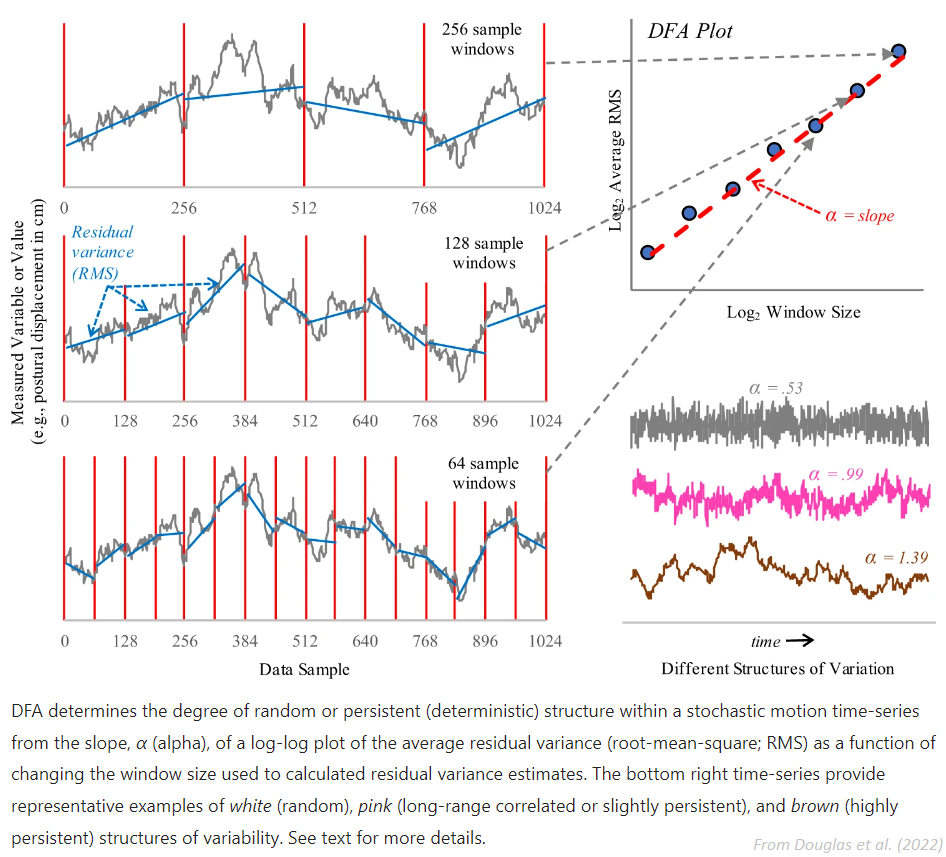
Detrended fluctuation analysis (DFA) is used to find long-term statistical dependencies in time series.

For monofractal DFA, the output alpha $\alpha$ corresponds to the slope of the linear trend between the scale factors and the fluctuations. For multifractal DFA, the slope values under different q values are actually generalised Hurst exponents h. Monofractal DFA corresponds to MFDFA with q = 2, and its output is actually an estimation of the Hurst exponent ($h_{(2)}$).

The Hurst exponent is the measure of long range autocorrelation of a signal, and $h_{(2)} > 0.5$ suggests the presence of long range correlation, while $h_{(2)} < 0.5`suggests short range correlations. If :math:`h_{(2)} = 0.5$, it indicates uncorrelated indiscriminative fluctuations, i.e. a Brownian motion.

Illustration of DFA (Douglas et al., 2022).

Multifractal DFA returns the generalised Hurst exponents h for different values of q. It is converted to the multifractal scaling exponent Tau $\tau_{(q)}$, which non-linear relationship with q can indicate multifractility. From there, we derive the singularity exponent H (or $\alpha$) (also known as Hölder’s exponents) and the singularity dimension D (or $f(\alpha)$). The variation of D with H is known as multifractal singularity spectrum (MSP), and usually has shape of an inverted parabola. It measures the long range correlation property of a signal. From these elements, different features are extracted:

Width: The width of the singularity spectrum, which quantifies the degree of the multifractality. In the case of monofractal signals, the MSP width is zero, since h(q) is independent of q.
Peak: The value of the singularity exponent H corresponding to the peak of singularity dimension D. It is a measure of the self-affinity of the signal, and a high value is an indicator of high degree of correlation between the data points. In the other words, the process is recurrent and repetitive.
Mean: The mean of the maximum and minimum values of singularity exponent H, which quantifies the average fluctuations of the signal.
Max: The value of singularity spectrum D corresponding to the maximum value of singularity exponent H, which indicates the maximum fluctuation of the signal.
Delta: the vertical distance between the singularity spectrum D where the singularity exponents are at their minimum and maximum. Corresponds to the range of fluctuations of the signal.
Asymmetry: The Asymmetric Ratio (AR) corresponds to the centrality of the peak of the spectrum. AR = 0.5 indicates that the multifractal spectrum is symmetric (Orozco-Duque et al., 2015).
Fluctuation: The h-fluctuation index (hFI) is defined as the power of the second derivative of h(q). See Orozco-Duque et al. (2015).
Increment: The cumulative function of the squared increments ($\alpha CF$) of the generalized Hurst’s exponents between consecutive moment orders is a more robust index of the distribution of the generalized Hurst’s exponents (Faini et al., 2021).

This function can be called either via fractal_dfa() or complexity_dfa(), and its multifractal variant can be directly accessed via fractal_mfdfa() or complexity_mfdfa().

Note

Help is needed to implement the modified formula to compute the slope when q = 0. See for instance Faini et al. (2021). See LRydin/MFDFA#33

Parameters:

signal (Union[list, np.array, pd.Series]) – The signal (i.e., a time series) in the form of a vector of values.
scale (list) – A list containing the lengths of the windows (number of data points in each subseries) that the signal is divided into. Also referred to as Tau $\tau$. If "default", will set it to a logarithmic scale (so that each window scale has the same weight) with a minimum of 4 and maximum of a tenth of the length (to have more than 10 windows to calculate the average fluctuation).
overlap (bool) – Defaults to True, where the windows will have a 50% overlap with each other, otherwise non-overlapping windows will be used.
integrate (bool) – It is common practice to convert the signal to a random walk (i.e., detrend and integrate, which corresponds to the signal ‘profile’) in order to avoid having too small exponent values. Note that it leads to the flattening of the signal, which can lead to the loss of some details (see Ihlen, 2012 for an explanation). Note that for strongly anticorrelated signals, this transformation should be applied two times (i.e., provide np.cumsum(signal - np.mean(signal)) instead of signal).
order (int) – The order of the polynomial trend for detrending. 1 corresponds to a linear detrending.
multifractal (bool) – If True, compute Multifractal Detrended Fluctuation Analysis (MFDFA), in which case the argument q is taken into account.
q (Union[int, list, np.array]) – The sequence of fractal exponents when multifractal=True. Must be a sequence between -10 and 10 (note that zero will be removed, since the code does not converge there). Setting q = 2 (default for DFA) gives a result of a standard DFA. For instance, Ihlen (2012) uses q = [-5, -3, -1, 0, 1, 3, 5] (default when for multifractal). In general, positive q moments amplify the contribution of fractal components with larger amplitude and negative q moments amplify the contribution of fractal with smaller amplitude (Kantelhardt et al., 2002).
maxdfa (bool) – If True, it will locate the knee of the fluctuations (using find_knee()) and use that as a maximum scale value. It computes max. DFA (a similar method exists in entropy_rate()).
show (bool) – Visualise the trend between the window size and the fluctuations.
**kwargs (optional) – Currently not used.

Returns:

dfa (float or pd.DataFrame) – If multifractal is False, one DFA value is returned for a single time series.
parameters (dict) – A dictionary containing additional information regarding the parameters used to compute DFA. If multifractal is False, the dictionary contains q value, a series of windows, fluctuations of each window and the slopes value of the log2(windows) versus log2(fluctuations) plot. If multifractal is True, the dictionary additionally contains the parameters of the singularity spectrum.

Examples

Example 1: Monofractal DFA

In [1]: import neurokit2 as nk

In [2]: signal = nk.signal_simulate(duration=10, frequency=[5, 7, 10, 14], noise=0.05)

In [3]: dfa, info = nk.fractal_dfa(signal, show=True)

$savefig/p_fractal_dfa1.png$

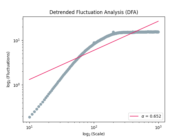
In [4]: dfa
Out[4]: 0.6490386114165136

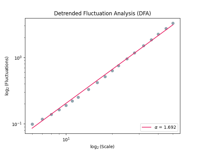
As we can see from the plot, the final value, corresponding to the slope of the red line, doesn’t capture properly the relationship. We can adjust the scale factors to capture the fractality of short-term fluctuations.

In [5]: scale = nk.expspace(10, 100, 20, base=2)

In [6]: dfa, info = nk.fractal_dfa(signal, scale=scale, show=True)

$savefig/p_fractal_dfa2.png$

Example 2: Multifractal DFA (MFDFA)

In [7]: mfdfa, info = nk.fractal_mfdfa(signal, q=[-5, -3, -1, 0, 1, 3, 5], show=True)

$savefig/p_fractal_dfa3.png$

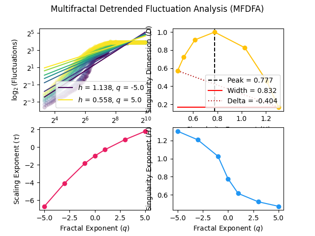
In [8]: mfdfa
Out[8]: 
      Width     Peak      Mean  ...  Asymmetry  Fluctuation  Increment
0  0.809923  0.77076  0.875426  ...   -0.37077     0.000219   0.038554

[1 rows x 8 columns]

References

Faini, A., Parati, G., & Castiglioni, P. (2021). Multiscale assessment of the degree of multifractality for physiological time series. Philosophical Transactions of the Royal Society A, 379(2212), 20200254.
Orozco-Duque, A., Novak, D., Kremen, V., & Bustamante, J. (2015). Multifractal analysis for grading complex fractionated electrograms in atrial fibrillation. Physiological Measurement, 36(11), 2269-2284.
Ihlen, E. A. F. E. (2012). Introduction to multifractal detrended fluctuation analysis in Matlab. Frontiers in physiology, 3, 141.
Kantelhardt, J. W., Zschiegner, S. A., Koscielny-Bunde, E., Havlin, S., Bunde, A., & Stanley, H. E. (2002). Multifractal detrended fluctuation analysis of nonstationary time series. Physica A: Statistical Mechanics and its Applications, 316(1-4), 87-114.
Hardstone, R., Poil, S. S., Schiavone, G., Jansen, R., Nikulin, V. V., Mansvelder, H. D., & Linkenkaer-Hansen, K. (2012). Detrended fluctuation analysis: a scale-free view on neuronal oscillations. Frontiers in physiology, 3, 450.

fractal_tmf()#

fractal_tmf(signal, n=40, show=False, **kwargs)[source]#

Multifractal Nonlinearity (tMF)

The Multifractal Nonlinearity index (tMF) is the t-value resulting from the comparison of the multifractality of the signal (measured by the spectrum width, see fractal_dfa()) with the multifractality of linearized surrogates obtained by the IAAFT method (i.e., reshuffled series with comparable linear structure).

This statistics grows larger the more the original series departs from the multifractality attributable to the linear structure of IAAFT surrogates. When p-value reaches significance, we can conclude that the signal’s multifractality encodes processes that a linear contingency cannot.

This index provides an extension of the assessment of multifractality, of which the multifractal spectrum is by itself a measure of heterogeneity, rather than interactivity. As such, it cannot alone be used to assess the specific presence of cascade-like interactivity in the time series, but must be compared to the spectrum of a sample of its surrogates.

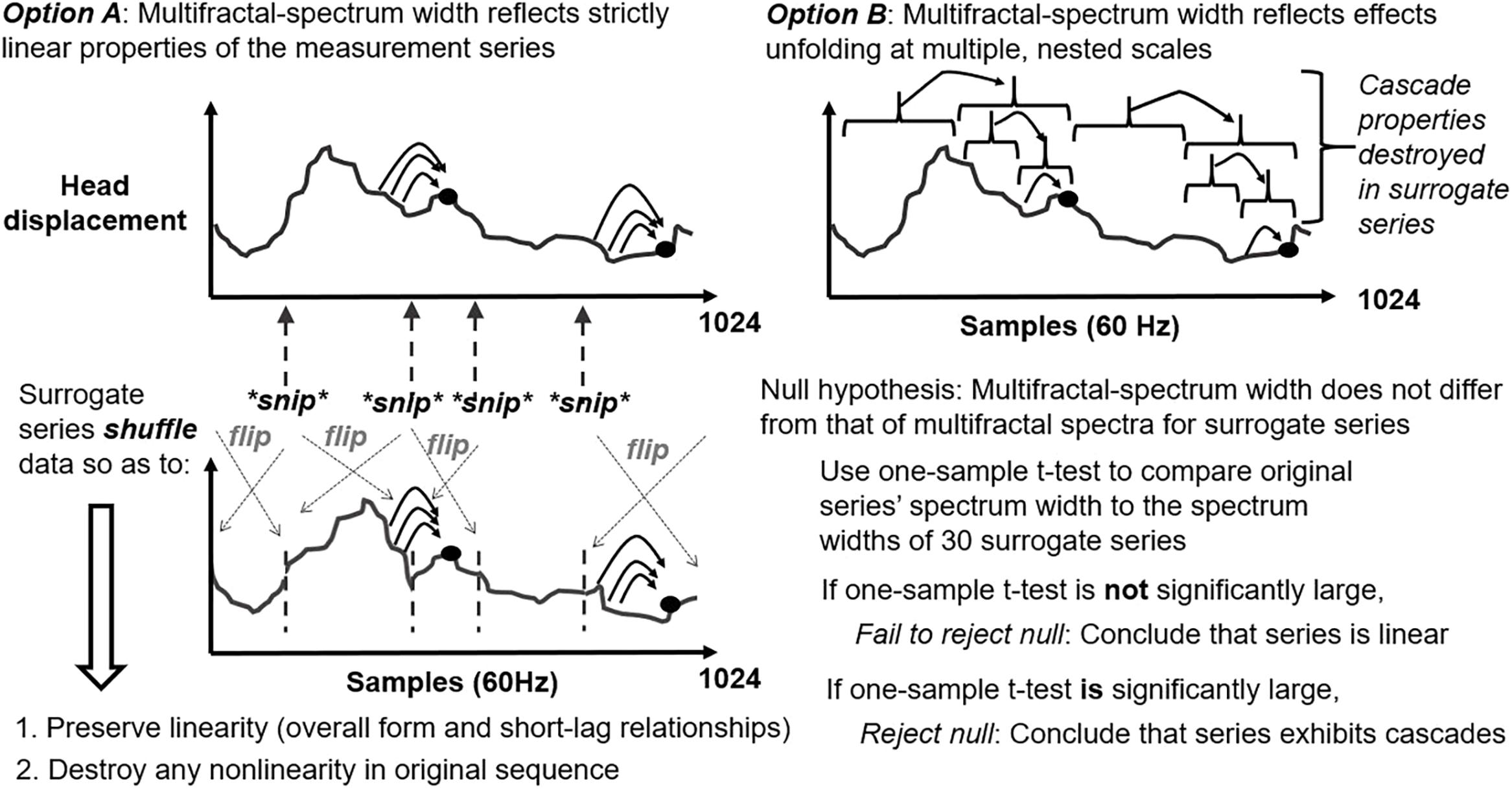
Both significantly negative and positive values can indicate interactivity, as any difference from the linear structure represented by the surrogates is an indication of nonlinear contingence. Indeed, if the degree of heterogeneity for the original series is significantly less than for the sample of linear surrogates, that is no less evidence of a failure of linearity than if the degree of heterogeneity is significantly greater.

Note

Help us review the implementation of this index by checking-it out and letting us know wether it is correct or not.

Parameters:

signal (Union[list, np.array, pd.Series]) – The signal (i.e., a time series) in the form of a vector of values.
n (int) – Number of surrogates. The literature uses values between 30 and 40.
**kwargs (optional) – Other arguments to be passed to fractal_dfa().

Returns:

float – tMF index.
info (dict) – A dictionary containing additional information, such as the p-value.

See also

fractal_dfa, signal_surrogate

Examples

In [1]: import neurokit2 as nk

# Simulate a Signal
In [2]: signal = nk.signal_simulate(duration=1, sampling_rate=200, frequency=[5, 6, 12], noise=0.2)

# Compute tMF
In [3]: tMF, info = nk.fractal_tmf(signal, n=100, show=True)

$savefig/p_fractal_tmf.png$

In [4]: tMF  # t-value
Out[4]: -3.6662392100069088

In [5]: info["p"]  # p-value
Out[5]: 0.0003981140698786622

References

Ihlen, E. A., & Vereijken, B. (2013). Multifractal formalisms of human behavior. Human movement science, 32(4), 633-651.
Kelty-Stephen, D. G., Palatinus, K., Saltzman, E., & Dixon, J. A. (2013). A tutorial on multifractality, cascades, and interactivity for empirical time series in ecological science. Ecological Psychology, 25(1), 1-62.
Bell, C. A., Carver, N. S., Zbaracki, J. A., & Kelty-Stephen, D. G. (2019). Non-linear amplification of variability through interaction across scales supports greater accuracy in manual aiming: evidence from a multifractal analysis with comparisons to linear surrogates in the fitts task. Frontiers in physiology, 10, 998.

Entropy#

entropy_shannon()#

entropy_shannon(signal=None, base=2, symbolize=None, show=False, freq=None, **kwargs)[source]#

Shannon entropy (SE or ShanEn)

Compute Shannon entropy (SE). Entropy is a measure of unpredictability of the state, or equivalently, of its average information content. Shannon entropy (SE) is one of the first and most basic measures of entropy and a foundational concept of information theory, introduced by Shannon (1948) to quantify the amount of information in a variable.

\[ShanEn = -\sum_{x \in \mathcal{X}} p(x) \log_2 p(x)\]

Shannon attempted to extend Shannon entropy in what has become known as Differential Entropy (see entropy_differential()).

Because Shannon entropy was meant for symbolic sequences (discrete events such as [“A”, “B”, “B”, “A”]), it does not do well with continuous signals. One option is to binarize (i.e., cut) the signal into a number of bins using for instance pd.cut(signal, bins=100, labels=False). This can be done automatically using the method argument, which will be transferred to complexity_symbolize().

This function can be called either via entropy_shannon() or complexity_se().

Parameters:

signal (Union[list, np.array, pd.Series]) – The signal (i.e., a time series) in the form of a vector of values.
base (float) – The logarithmic base to use, defaults to 2, giving a unit in bits. Note that scipy. stats.entropy() uses Euler’s number (np.e) as default (the natural logarithm), giving a measure of information expressed in nats.
symbolize (str) – Method to convert a continuous signal input into a symbolic (discrete) signal. None by default, which skips the process (and assumes the input is already discrete). See complexity_symbolize() for details.
show (bool) – If True, will show the discrete the signal.
freq (np.array) – Instead of a signal, a vector of probabilities can be provided (used for instance in entropy_permutation()).
**kwargs – Optional arguments. Not used for now.

Returns:

shanen (float) – The Shannon entropy of the signal.
info (dict) – A dictionary containing additional information regarding the parameters used to compute Shannon entropy.

Examples

In [1]: import neurokit2 as nk

In [2]: signal = [1, 1, 5, 5, 2, 8, 1]

In [3]: _, freq = np.unique(signal, return_counts=True)

In [4]: nk.entropy_shannon(freq=freq)
Out[4]: (1.8423709931771086, {'Symbolization': None, 'Base': 2})

# Simulate a Signal with Laplace Noise
In [5]: signal = nk.signal_simulate(duration=2, frequency=5, noise=0.01)

# Compute Shannon's Entropy
In [6]: shanen, info = nk.entropy_shannon(signal, symbolize=3, show=True)

In [7]: shanen
Out[7]: 1.5516176235074324

Compare with scipy (using the same base).

In [8]: import scipy.stats

# Make the binning ourselves
In [9]: binned = pd.cut(signal, bins=3, labels=False)

In [10]: scipy.stats.entropy(pd.Series(binned).value_counts())
Out[10]: 1.0754993810412994

In [11]: shanen, info = nk.entropy_shannon(binned, base=np.e)

In [12]: shanen
Out[12]: 1.0754993810412994

References

Shannon, C. E. (1948). A mathematical theory of communication. The Bell system technical journal, 27(3), 379-423.

entropy_maximum()#

entropy_maximum(signal)[source]#

Maximum Entropy (MaxEn)

Provides an upper bound for the entropy of a random variable, so that the empirical entropy (obtained for instance with entropy_shannon()) will lie in between 0 and max. entropy.

It can be useful to normalize the empirical entropy by the maximum entropy (which is made by default in some algorithms).

Parameters:

signal (Union[list, np.array, pd.Series]) – The signal (i.e., a time series) in the form of a vector of values.

Returns:

maxen (float) – The maximum entropy of the signal.
info (dict) – An empty dictionary returned for consistency with the other complexity functions.

See also

entropy_shannon

Examples

In [1]: import neurokit2 as nk

In [2]: signal = [1, 1, 5, 5, 2, 8, 1]

In [3]: maxen, _ = nk.entropy_maximum(signal)

In [4]: maxen
Out[4]: 2.0

entropy_differential()#

entropy_differential(signal, base=2, **kwargs)[source]#

Differential entropy (DiffEn)

Differential entropy (DiffEn; also referred to as continuous entropy) started as an attempt by Shannon to extend Shannon entropy. However, differential entropy presents some issues too, such as that it can be negative even for simple distributions (such as the uniform distribution).

This function can be called either via entropy_differential() or complexity_diffen().

Parameters:

signal (Union[list, np.array, pd.Series]) – The signal (i.e., a time series) in the form of a vector of values.
base (float) – The logarithmic base to use, defaults to 2, giving a unit in bits. Note that scipy. stats.entropy() uses Euler’s number (np.e) as default (the natural logarithm), giving a measure of information expressed in nats.
**kwargs (optional) – Other arguments passed to scipy.stats.differential_entropy().

Returns:

diffen (float) – The Differential entropy of the signal.
info (dict) – A dictionary containing additional information regarding the parameters used to compute Differential entropy.

Examples

In [1]: import neurokit2 as nk

# Simulate a Signal with Laplace Noise
In [2]: signal = nk.signal_simulate(duration=2, frequency=5, noise=0.1)

# Compute Differential Entropy
In [3]: diffen, info = nk.entropy_differential(signal)

In [4]: diffen
Out[4]: 0.5225147355234878

References

entropy_power()#

entropy_power(signal, **kwargs)[source]#

Entropy Power (PowEn)

The Shannon Entropy Power (PowEn or SEP) is a measure of the effective variance of a random vector. It is based on the estimation of the density of the variable, thus relying on density().

Warning

We are not sure at all about the correct implementation of this function. Please consider helping us by double-checking the code against the formulas in the references.

Parameters:

signal (Union[list, np.array, pd.Series]) – The signal (i.e., a time series) in the form of a vector of values.
**kwargs – Other arguments to be passed to density_bandwidth().

Returns:

powen (float) – The computed entropy power measure.
info (dict) – A dictionary containing additional information regarding the parameters used.

See also

information_fisershannon

Examples

In [1]: import neurokit2 as nk

In [2]: import matplotlib.pyplot as plt

In [3]: signal = nk.signal_simulate(duration=10, frequency=[10, 12], noise=0.1)

In [4]: powen, info = nk.entropy_power(signal)

In [5]: powen
Out[5]: 0.058559168114939504

# Visualize the distribution that the entropy power is based on
In [6]: plt.plot(info["Values"], info["Density"])
Out[6]: [<matplotlib.lines.Line2D at 0x255c4115660>]

Change density bandwidth.

In [7]: powen, info = nk.entropy_power(signal, bandwidth=0.01)

In [8]: powen
Out[8]: 0.058558940287037176

References

Guignard, F., Laib, M., Amato, F., & Kanevski, M. (2020). Advanced analysis of temporal data using Fisher-Shannon information: theoretical development and application in geosciences. Frontiers in Earth Science, 8, 255.
Vignat, C., & Bercher, J. F. (2003). Analysis of signals in the Fisher-Shannon information plane. Physics Letters A, 312(1-2), 27-33.
Dembo, A., Cover, T. M., & Thomas, J. A. (1991). Information theoretic inequalities. IEEE Transactions on Information theory, 37(6), 1501-1518.

entropy_tsallis()#

entropy_tsallis(signal=None, q=1, symbolize=None, show=False, freq=None, **kwargs)[source]#

Tsallis entropy (TSEn)

Tsallis Entropy is an extension of Shannon entropy to the case where entropy is nonextensive. It is similarly computed from a vector of probabilities of different states. Because it works on discrete inputs (e.g., [A, B, B, A, B]), it requires to transform the continuous signal into a discrete one.

\[TSEn = \frac{1}{q - 1} \left( 1 - \sum_{x \in \mathcal{X}} p(x)^q \right)\]

Parameters:

signal (Union[list, np.array, pd.Series]) – The signal (i.e., a time series) in the form of a vector of values.
q (float) – Tsallis’s q parameter, sometimes referred to as the entropic-index (default to 1).
symbolize (str) – Method to convert a continuous signal input into a symbolic (discrete) signal. None by default, which skips the process (and assumes the input is already discrete). See complexity_symbolize() for details.
show (bool) – If True, will show the discrete the signal.
freq (np.array) – Instead of a signal, a vector of probabilities can be provided.
**kwargs – Optional arguments. Not used for now.

Returns:

tsen (float) – The Tsallis entropy of the signal.
info (dict) – A dictionary containing additional information regarding the parameters used.

Examples

In [1]: import neurokit2 as nk

In [2]: signal = [1, 3, 3, 2, 6, 6, 6, 1, 0]

In [3]: tsen, _ = nk.entropy_tsallis(signal, q=1)

In [4]: tsen
Out[4]: 1.5229550675313184

In [5]: shanen, _ = nk.entropy_shannon(signal, base=np.e)

In [6]: shanen
Out[6]: 1.5229550675313184

References

Tsallis, C. (2009). Introduction to nonextensive statistical mechanics: approaching a complex world. Springer, 1(1), 2-1.

entropy_renyi()#

entropy_renyi(signal=None, alpha=1, symbolize=None, show=False, freq=None, **kwargs)[source]#

Rényi entropy (REn or H)

In information theory, the Rényi entropy H generalizes the Hartley entropy, the Shannon entropy, the collision entropy and the min-entropy.

$\alpha = 0$: the Rényi entropy becomes what is known as the Hartley entropy.
$\alpha = 1$: the Rényi entropy becomes the :func:`Shannon entropy <entropy_shannon>`.
$\alpha = 2$: the Rényi entropy becomes the collision entropy, which corresponds to the surprisal of “rolling doubles”.

It is mathematically defined as:

\[REn = \frac{1}{1-\alpha} \log_2 \left( \sum_{x \in \mathcal{X}} p(x)^\alpha \right)\]

Parameters:

signal (Union[list, np.array, pd.Series]) – The signal (i.e., a time series) in the form of a vector of values.
alpha (float) – The alpha $\alpha$ parameter (default to 1) for Rényi entropy.
symbolize (str) – Method to convert a continuous signal input into a symbolic (discrete) signal. None by default, which skips the process (and assumes the input is already discrete). See complexity_symbolize() for details.
show (bool) – If True, will show the discrete the signal.
freq (np.array) – Instead of a signal, a vector of probabilities can be provided.
**kwargs – Optional arguments. Not used for now.

Returns:

ren (float) – The Tsallis entropy of the signal.
info (dict) – A dictionary containing additional information regarding the parameters used.

See also

entropy_shannon, entropy_tsallis

Examples

In [1]: import neurokit2 as nk

In [2]: signal = [1, 3, 3, 2, 6, 6, 6, 1, 0]

In [3]: tsen, _ = nk.entropy_renyi(signal, alpha=1)

In [4]: tsen
Out[4]: 1.5229550675313184

# Compare to Shannon function
In [5]: shanen, _ = nk.entropy_shannon(signal, base=np.e)

In [6]: shanen
Out[6]: 1.5229550675313184

# Hartley Entropy
In [7]: nk.entropy_renyi(signal, alpha=0)[0]
Out[7]: 1.6094379124341003

# Collision Entropy
In [8]: nk.entropy_renyi(signal, alpha=2)[0]
Out[8]: 1.4500101755059984

References

Rényi, A. (1961, January). On measures of entropy and information. In Proceedings of the Fourth Berkeley Symposium on Mathematical Statistics and Probability, Volume 1: Contributions to the Theory of Statistics (Vol. 4, pp. 547-562). University of California Press.

entropy_approximate()#

entropy_approximate(signal, delay=1, dimension=2, tolerance='sd', corrected=False, **kwargs)[source]#

Approximate entropy (ApEn) and its corrected version (cApEn)

Approximate entropy is a technique used to quantify the amount of regularity and the unpredictability of fluctuations over time-series data. The advantages of ApEn include lower computational demand (ApEn can be designed to work for small data samples (< 50 data points) and can be applied in real time) and less sensitive to noise. However, ApEn is heavily dependent on the record length and lacks relative consistency.

This function can be called either via entropy_approximate() or complexity_apen(), and the corrected version via complexity_capen().

Parameters:

signal (Union[list, np.array, pd.Series]) – The signal (i.e., a time series) in the form of a vector of values.
delay (int) – Time delay (often denoted Tau $\tau$, sometimes referred to as lag) in samples. See complexity_delay() to estimate the optimal value for this parameter.
dimension (int) – Embedding Dimension (m, sometimes referred to as d or order). See complexity_dimension() to estimate the optimal value for this parameter.
tolerance (float) – Tolerance (often denoted as r), distance to consider two data points as similar. If "sd" (default), will be set to $0.2 * SD_{signal}$. See complexity_tolerance() to estimate the optimal value for this parameter.
corrected (bool) – If true, will compute corrected ApEn (cApEn), see Porta (2007).
**kwargs – Other arguments.

Returns:

apen (float) – The approximate entropy of the single time series.
info (dict) – A dictionary containing additional information regarding the parameters used to compute approximate entropy.

Examples

In [1]: import neurokit2 as nk

In [2]: signal = nk.signal_simulate(duration=2, frequency=5)

In [3]: apen, parameters = nk.entropy_approximate(signal)

In [4]: apen
Out[4]: 0.08837414074679684

In [5]: capen, parameters = nk.entropy_approximate(signal, corrected=True)

In [6]: capen
Out[6]: 0.08907775138332998

References

Sabeti, M., Katebi, S., & Boostani, R. (2009). Entropy and complexity measures for EEG signal classification of schizophrenic and control participants. Artificial intelligence in medicine, 47(3), 263-274.
Shi, B., Zhang, Y., Yuan, C., Wang, S., & Li, P. (2017). Entropy analysis of short-term heartbeat interval time series during regular walking. Entropy, 19(10), 568.

entropy_sample()#

entropy_sample(signal, delay=1, dimension=2, tolerance='sd', **kwargs)[source]#

Sample Entropy (SampEn)

Compute the sample entropy (SampEn) of a signal. SampEn is a modification of ApEn used for assessing complexity of physiological time series signals. It corresponds to the conditional probability that two vectors that are close to each other for m dimensions will remain close at the next m + 1 component.

This function can be called either via entropy_sample() or complexity_sampen().

Parameters:

signal (Union[list, np.array, pd.Series]) – The signal (i.e., a time series) in the form of a vector of values.
delay (int) – Time delay (often denoted Tau $\tau$, sometimes referred to as lag) in samples. See complexity_delay() to estimate the optimal value for this parameter.
dimension (int) – Embedding Dimension (m, sometimes referred to as d or order). See complexity_dimension() to estimate the optimal value for this parameter.
tolerance (float) – Tolerance (often denoted as r), distance to consider two data points as similar. If "sd" (default), will be set to $0.2 * SD_{signal}$. See complexity_tolerance() to estimate the optimal value for this parameter.
**kwargs (optional) – Other arguments.

Returns:

sampen (float) – The sample entropy of the single time series. If undefined conditional probabilities are detected (logarithm of sum of conditional probabilities is ln(0)), np.inf will be returned, meaning it fails to retrieve ‘accurate’ regularity information. This tends to happen for short data segments, increasing tolerance levels might help avoid this.
info (dict) – A dictionary containing additional information regarding the parameters used to compute sample entropy.

Examples

In [1]: import neurokit2 as nk

In [2]: signal = nk.signal_simulate(duration=2, frequency=5)

In [3]: sampen, parameters = nk.entropy_sample(signal, delay=1, dimension=2)

In [4]: sampen
Out[4]: 0.07380851770121913

entropy_quadratic()#

entropy_quadratic(signal, delay=1, dimension=2, tolerance='sd', **kwargs)[source]#

Quadratic Sample Entropy (QSE)

Compute the quadratic sample entropy (QSE) of a signal. It is essentially a correction of SampEn introduced by Lake (2005) defined as:

\[QSE = SampEn + ln(2 * tolerannce)\]

QSE has been described as a more stable measure of entropy than SampEn (Gylling, 2017).

Parameters:

signal (Union[list, np.array, pd.Series]) – The signal (i.e., a time series) in the form of a vector of values.
delay (int) – Time delay (often denoted Tau $\tau$, sometimes referred to as lag) in samples. See complexity_delay() to estimate the optimal value for this parameter.
dimension (int) – Embedding Dimension (m, sometimes referred to as d or order). See complexity_dimension() to estimate the optimal value for this parameter.
tolerance (float) – Tolerance (often denoted as r), distance to consider two data points as similar. If "sd" (default), will be set to $0.2 * SD_{signal}$. See complexity_tolerance() to estimate the optimal value for this parameter.
**kwargs (optional) – Other arguments.

See also

entropy_sample

Returns:

qse (float) – The uadratic sample entropy of the single time series.
info (dict) – A dictionary containing additional information regarding the parameters used to compute sample entropy.

Examples

In [1]: import neurokit2 as nk

In [2]: signal = nk.signal_simulate(duration=2, frequency=5)

In [3]: qsa, parameters = nk.entropy_quadratic(signal, delay=1, dimension=2)

In [4]: qsa
Out[4]: -1.8819529224920126

References

Huselius Gylling, K. (2017). Quadratic sample entropy as a measure of burstiness: A study in how well Rényi entropy rate and quadratic sample entropy can capture the presence of spikes in time-series data.
Lake, D. E. (2005). Renyi entropy measures of heart rate Gaussianity. IEEE Transactions on Biomedical Engineering, 53(1), 21-27.

entropy_cumulativeresidual()#

entropy_cumulativeresidual(signal, symbolize=None, show=False, freq=None)[source]#

Cumulative residual entropy (CREn)

The cumulative residual entropy is an alternative to the Shannon differential entropy with several advantageous properties, such as non-negativity. The key idea is to use the cumulative distribution (CDF) instead of the density function in Shannon’s entropy.

\[CREn = -\int_{0}^{\infty} p(|X| > x) \log_{2} p(|X| > x) dx\]

Similarly to Shannon entropy and Petrosian fractal dimension, different methods to transform continuous signals into discrete ones are available. See complexity_symbolize() for details.

This function can be called either via entropy_cumulativeresidual() or complexity_cren().

Parameters:

signal (Union[list, np.array, pd.Series]) – The signal (i.e., a time series) in the form of a vector of values.
symbolize (str) – Method to convert a continuous signal input into a symbolic (discrete) signal. None by default, which skips the process (and assumes the input is already discrete). See complexity_symbolize() for details.
show (bool) – If True, will show the discrete the signal.
freq (np.array) – Instead of a signal, a vector of probabilities can be provided.

Returns:

CREn (float) – The cumulative residual entropy.
info (dict) – A dictionary containing Values for each pair of events.

Examples

In [1]: import neurokit2 as nk

In [2]: signal = [1, 1, 1, 3, 3, 2, 2, 1, 1, 3, 3, 3]

In [3]: cren, info = nk.entropy_cumulativeresidual(signal, show=True)

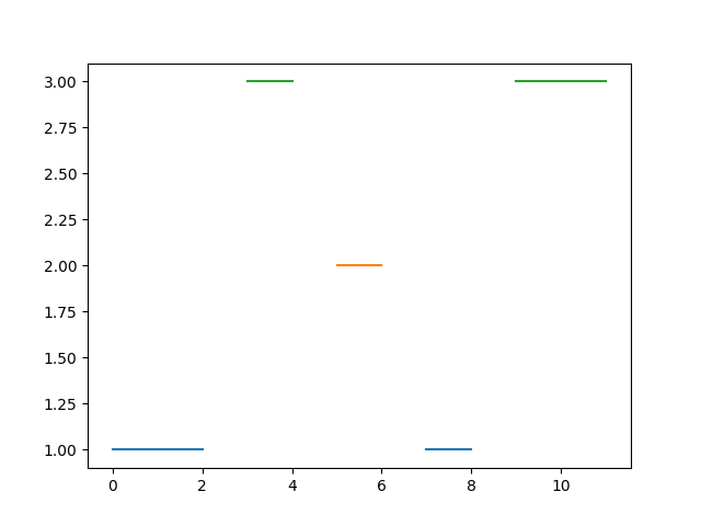
savefig/p_entropy_cumulativeresidual1.png

In [4]: cren
Out[4]: 0.9798687566511528

References

Rao, M., Chen, Y., Vemuri, B. C., & Wang, F. (2004). Cumulative residual entropy: a new measure of information. IEEE transactions on Information Theory, 50(6), 1220-1228.

entropy_rate()#

entropy_rate(signal, kmax=10, symbolize='mean', show=False)[source]#

Entropy Rate (RatEn)

The Entropy Rate (RatEn or ER) quantifies the amount of information needed to describe the signal given observations of signal(k). In other words, it is the entropy of the time series conditioned on the k-histories.

It quantifies how much uncertainty or randomness the process produces at each new time step, given knowledge about the past states of the process. The entropy rate is estimated as the slope of the linear fit between the history length k and the joint Shannon entropies. The entropy at k = 1 is called Excess Entropy (ExEn).

We adapted the algorithm to include a knee-point detection (beyond which the self-Entropy reaches a plateau), and if it exists, we additionally re-compute the Entropy Rate up until that point. This Maximum Entropy Rate (MaxRatEn) can be retrieved from the dictionary.

Parameters:

signal (Union[list, np.array, pd.Series]) – A symbolic sequence in the form of a vector of values.
kmax (int) – The max history length to consider. If an integer is passed, will generate a range from 1 to kmax.
symbolize (str) – Method to convert a continuous signal input into a symbolic (discrete) signal. By default, assigns 0 and 1 to values below and above the mean. Can be None to skip the process (in case the input is already discrete). See complexity_symbolize() for details.
show (bool) – Plot the Entropy Rate line.

See also

entropy_shannon

Examples

Example 1: A simple discrete signal. We have to specify symbolize=None as the signal is already discrete.

In [1]: import neurokit2 as nk

In [2]: signal = [1, 1, 2, 1, 2, 1, 1, 1, 2, 2, 1, 1, 1, 3, 2, 2, 1, 3, 2]

In [3]: raten, info = nk.entropy_rate(signal, kmax=10, symbolize=None, show=True)

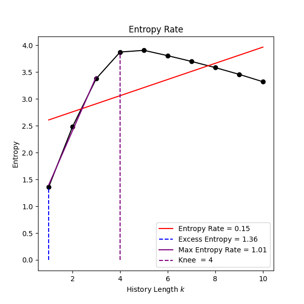
Here we can see that kmax is likely to big to provide an accurate estimation of entropy rate.

In [4]: raten, info = nk.entropy_rate(signal, kmax=3, symbolize=None, show=True)

Example 2: A continuous signal.

In [5]: signal = nk.signal_simulate(duration=2, frequency=[5, 12, 40, 60], sampling_rate=1000)

In [6]: raten, info = nk.entropy_rate(signal, kmax=60, show=True)

In [7]: raten
Out[7]: 0.13604346820833424

In [8]: info["Excess_Entropy"]
Out[8]: 0.9999971146079947

In [9]: info["MaxRatEn"]
Out[9]: 0.3211967949605768

References

Mediano, P. A., Rosas, F. E., Timmermann, C., Roseman, L., Nutt, D. J., Feilding, A., … & Carhart-Harris, R. L. (2020). Effects of external stimulation on psychedelic state neurodynamics. Biorxiv.

entropy_svd()#

entropy_svd(signal, delay=1, dimension=2, show=False)[source]#

Singular Value Decomposition (SVD) Entropy

SVD entropy (SVDEn) can be intuitively seen as an indicator of how many eigenvectors are needed for an adequate explanation of the dataset. In other words, it measures feature-richness: the higher the SVD entropy, the more orthogonal vectors are required to adequately explain the space-state. Similarly to Fisher Information (FI), it is based on the Singular Value Decomposition of the time-delay embedded signal.

Parameters:

signal (Union[list, np.array, pd.Series]) – The signal (i.e., a time series) in the form of a vector of values.
delay (int) – Time delay (often denoted Tau $\tau$, sometimes referred to as lag) in samples. See complexity_delay() to estimate the optimal value for this parameter.
dimension (int) – Embedding Dimension (m, sometimes referred to as d or order). See complexity_dimension() to estimate the optimal value for this parameter.
show (bool) – If True, will plot the attractor.

Returns:

svd (float) – The singular value decomposition (SVD).
info (dict) – A dictionary containing additional information regarding the parameters used to compute SVDEn.

Examples

In [1]: import neurokit2 as nk

In [2]: signal = nk.signal_simulate(duration=1, frequency=5)

In [3]: svden, info = nk.entropy_svd(signal, delay=5, dimension=3, show=True)

In [4]: svden
Out[4]: 0.5091667337544503

References

Roberts, S. J., Penny, W., & Rezek, I. (1999). Temporal and spatial complexity measures for electroencephalogram based brain-computer interfacing. Medical & biological engineering & computing, 37(1), 93-98.

entropy_kl()#

entropy_kl(signal, delay=1, dimension=2, norm='euclidean', **kwargs)[source]#

Kozachenko-Leonenko (K-L) Differential entropy (KLEn)

The Kozachenko-Leonenko (K-L) estimate of the differential entropy is also referred to as the nearest neighbor estimate of entropy.

Parameters:

signal (Union[list, np.array, pd.Series]) – The signal (i.e., a time series) in the form of a vector of values.
delay (int) – Time delay (often denoted Tau $\tau$, sometimes referred to as lag) in samples. See complexity_delay() to estimate the optimal value for this parameter.
dimension (int) – Embedding Dimension (m, sometimes referred to as d or order). See complexity_dimension() to estimate the optimal value for this parameter.
norm (str) – The probability norm used when computing k-nearest neighbour distances. Can be "euclidean" (default) or "max".
**kwargs (optional) – Other arguments (not used for now).

Returns:

klen (float) – The KL-entropy of the signal.
info (dict) – A dictionary containing additional information regarding the parameters used to compute Differential entropy.

See also

entropy_differential

Examples

In [1]: import neurokit2 as nk

# Simulate a Signal with Laplace Noise
In [2]: signal = nk.signal_simulate(duration=2, frequency=5, noise=0.1)

# Compute Kozachenko-Leonenko (K-L) Entropy
In [3]: klen, info = nk.entropy_kl(signal, delay=1, dimension=3)

In [4]: klen
Out[4]: 1.5742153436836026

References

Gautama, T., Mandic, D. P., & Van Hulle, M. M. (2003, April). A differential entropy based method for determining the optimal embedding parameters of a signal. In 2003 IEEE International Conference on Acoustics, Speech, and Signal Processing, 2003. Proceedings. (ICASSP’03). (Vol. 6, pp. VI-29). IEEE.
Beirlant, J., Dudewicz, E. J., Györfi, L., & Van der Meulen, E. C. (1997). Nonparametric entropy estimation: An overview. International Journal of Mathematical and Statistical Sciences, 6(1), 17-39.
Kozachenko, L., & Leonenko, N. (1987). Sample estimate of the entropy of a random vector. Problemy Peredachi Informatsii, 23(2), 9-16.

entropy_spectral()#

entropy_spectral(signal, bins=None, show=False, **kwargs)[source]#

Spectral Entropy (SpEn)

Spectral entropy (SE or SpEn) treats the signal’s normalized power spectrum density (PSD) in the frequency domain as a probability distribution, and calculates the Shannon entropy of it.

\[H(x, sf) = -\sum P(f) \log_2[P(f)]\]

A signal with a single frequency component (i.e., pure sinusoid) produces the smallest entropy. On the other hand, a signal with all frequency components of equal power value (white noise) produces the greatest entropy.

Parameters:

signal (Union[list, np.array, pd.Series]) – The signal (i.e., a time series) in the form of a vector of values.
bins (int) – If an integer is passed, will cut the PSD into a number of bins of frequency.
show (bool) – Display the power spectrum.
**kwargs (optional) – Keyword arguments to be passed to signal_psd().

Returns:

SpEn (float) – Spectral Entropy
info (dict) – A dictionary containing additional information regarding the parameters used.

See also

entropy_shannon, entropy_wiener, signal_psd

Examples

In [1]: import neurokit2 as nk

# Simulate a Signal with Laplace Noise
In [2]: signal = nk.signal_simulate(duration=2, sampling_rate=200, frequency=[5, 6, 10], noise=0.1)

# Compute Spectral Entropy
In [3]: SpEn, info = nk.entropy_spectral(signal, show=True)

In [4]: SpEn
Out[4]: 0.5974644455730078

Bin the frequency spectrum.

In [5]: SpEn, info = nk.entropy_spectral(signal, bins=10, show=True)

References

Crepeau, J. C., & Isaacson, L. K. (1991). Spectral Entropy Measurements of Coherent Structures in an Evolving Shear Layer. Journal of Non-Equilibrium Thermodynamics, 16(2). doi:10.1515/jnet.1991.16.2.137

entropy_phase()#

entropy_phase(signal, delay=1, k=4, show=False, **kwargs)[source]#

Phase Entropy (PhasEn)

Phase entropy (PhasEn or PhEn) has been developed by quantifying the distribution of the signal in accross k parts (of a two-dimensional phase space referred to as a second order difference plot (SODP). It build on the concept of Grid Entropy, that uses Poincaré plot as its basis.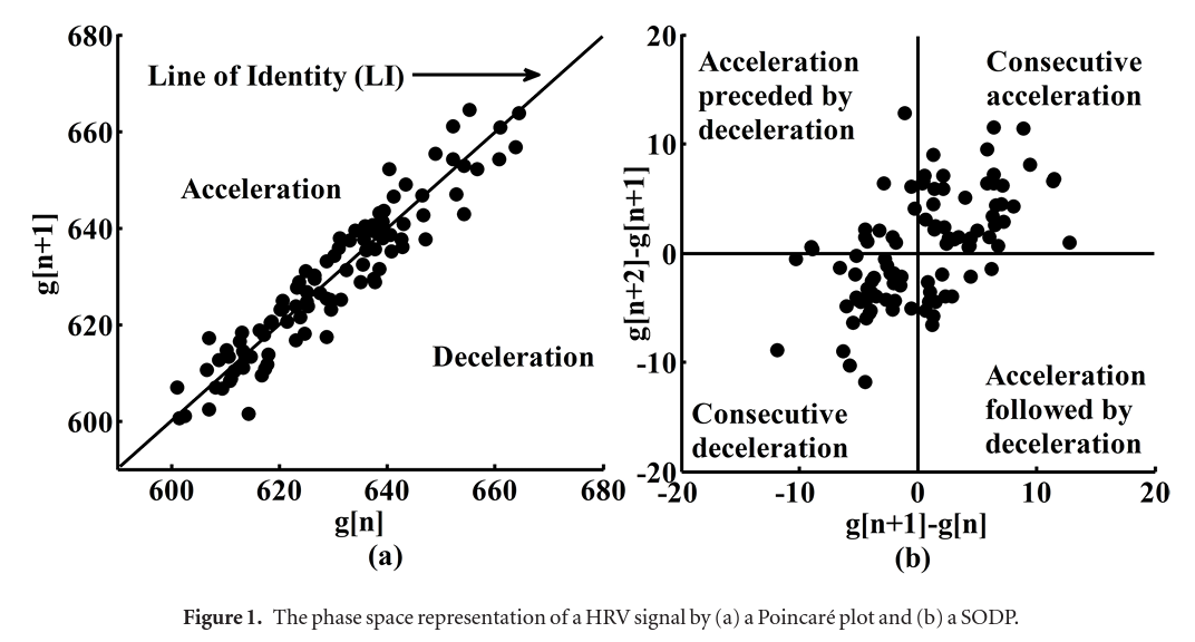

Parameters:

signal (Union[list, np.array, pd.Series]) – The signal (i.e., a time series) in the form of a vector of values.
delay (int) – Time delay (often denoted Tau $\tau$, sometimes referred to as lag) in samples. See complexity_delay() to estimate the optimal value for this parameter.
k (int) – The number of sections that the SODP is divided into. It is a coarse graining parameter that defines how fine the grid is. It is recommended to use even-numbered (preferably multiples of 4) partitions for sake of symmetry.
show (bool) – Plot the Second Order Difference Plot (SODP).
**kwargs (optional) – Other keyword arguments, such as the logarithmic base to use for entropy_shannon().

Returns:

phasen (float) – Phase Entropy
info (dict) – A dictionary containing additional information regarding the parameters used.

See also

entropy_shannon

Examples

In [1]: import neurokit2 as nk

# Simulate a Signal
In [2]: signal = nk.signal_simulate(duration=2, sampling_rate=200, frequency=[5, 6], noise=0.5)

# Compute Phase Entropy
In [3]: phasen, info = nk.entropy_phase(signal, k=4, show=True)

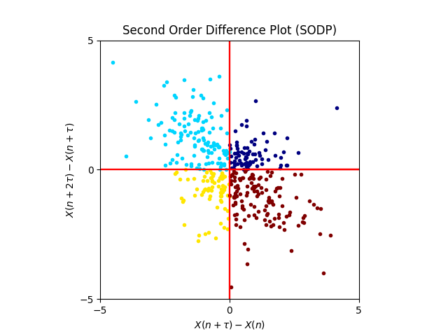
In [4]: phasen
Out[4]: 1.2027009809715699

In [5]: phasen, info = nk.entropy_phase(signal, k=8, show=True)

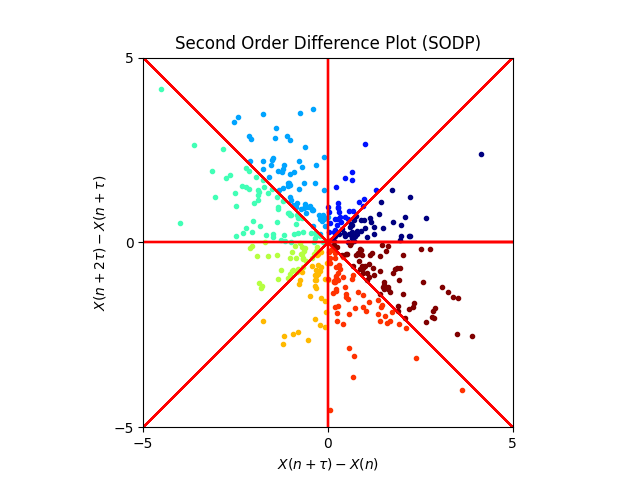
References

Rohila, A., & Sharma, A. (2019). Phase entropy: A new complexity measure for heart rate variability. Physiological Measurement, 40(10), 105006.

entropy_grid()#

entropy_grid(signal, delay=1, k=3, show=False, **kwargs)[source]#

Grid Entropy (GridEn)

Grid Entropy (GridEn or GDEn) is defined as a gridded descriptor of a Poincaré plot, which is a two-dimensional phase space diagram of a time series that plots the present sample of a time series with respect to their delayed values. The plot is divided into $n*n$ grids, and the Shannon entropy is computed from the probability distribution of the number of points in each grid.

Yan et al. (2019) define two novel measures, namely GridEn and Gridded Distribution Rate (GDR), the latter being the percentage of grids containing points.

Parameters:

signal (Union[list, np.array, pd.Series]) – The signal (i.e., a time series) in the form of a vector of values.
delay (int) – Time delay (often denoted Tau $\tau$, sometimes referred to as lag) in samples. See complexity_delay() to estimate the optimal value for this parameter.
k (int) – The number of sections that the Poincaré plot is divided into. It is a coarse graining parameter that defines how fine the grid is.
show (bool) – Plot the Poincaré plot.
**kwargs (optional) – Other keyword arguments, such as the logarithmic base to use for entropy_shannon().

Returns:

griden (float) – Grid Entropy of the signal.
info (dict) – A dictionary containing additional information regarding the parameters used.

Examples

In [1]: import neurokit2 as nk

# Simulate a Signal
In [2]: signal = nk.signal_simulate(duration=2, sampling_rate=200, frequency=[5, 6], noise=0.5)

# Compute Grid Entropy
In [3]: phasen, info = nk.entropy_grid(signal, k=3, show=True)

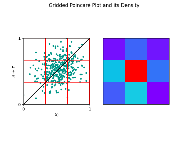
In [4]: phasen
Out[4]: 1.9113416673656225

In [5]: phasen, info = nk.entropy_grid(signal, k=10, show=True)

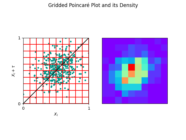
In [6]: info["GDR"]
Out[6]: 0.51

References

Yan, C., Li, P., Liu, C., Wang, X., Yin, C., & Yao, L. (2019). Novel gridded descriptors of poincaré plot for analyzing heartbeat interval time-series. Computers in biology and medicine, 109, 280-289.

entropy_attention()#

entropy_attention(signal, show=False, **kwargs)[source]#

Attention Entropy (AttEn)

Yang et al. (2020) propose a conceptually new approach called Attention Entropy (AttEn), which pays attention only to the key observations (local maxima and minima; i.e., peaks). Instead of counting the frequency of all observations, it analyzes the frequency distribution of the intervals between the key observations in a time-series. The advantages of the attention entropy are that it does not need any parameter to tune, is robust to the time-series length, and requires only linear time to compute.

Because this index relies on peak-detection, it is not suited for noisy signals. Signal cleaning (in particular filtering), and eventually more tuning for the peak detection algorithm, can help.

AttEn is computed as the average of various subindices, such as:

MaxMax: The entropy of local-maxima intervals.
MinMin: The entropy of local-minima intervals.
MaxMin: The entropy of intervals between local maxima and subsequent minima.
MinMax: The entropy of intervals between local minima and subsequent maxima.

Parameters:

signal (Union[list, np.array, pd.Series]) – The signal (i.e., a time series) in the form of a vector of values.
show (bool) – If True, the local maxima and minima will be displayed.

Returns:

atten (float) – The attention entropy of the signal.
info (dict) – A dictionary containing values of sub-entropies, such as MaxMax, MinMin, MaxMin, and MinMax.
**kwargs – Other arguments to be passed to scipy.signal.find_peaks().

See also

entropy_shannon, entropy_cumulative_residual

Examples

In [1]: import neurokit2 as nk

In [2]: signal = nk.signal_simulate(duration=1, frequency=5, noise=0.1)

# Compute Attention Entropy
In [3]: atten, info = nk.entropy_attention(signal, show=True)

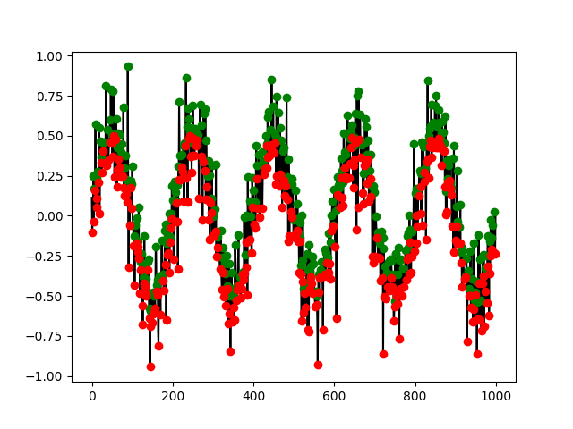
In [4]: atten
Out[4]: 1.0609206712571448

References

Yang, J., Choudhary, G. I., Rahardja, S., & Franti, P. (2020). Classification of interbeat interval time-series using attention entropy. IEEE Transactions on Affective Computing.

entropy_increment()#

entropy_increment(signal, dimension=2, q=4, **kwargs)[source]#

Increment Entropy (IncrEn) and its Multiscale variant (MSIncrEn)

Increment Entropy (IncrEn) quantifies the magnitudes of the variations between adjacent elements into ranks based on a precision factor q and the standard deviation of the time series. IncrEn is conceptually similar to permutation entropy in that it also uses the concepts of symbolic dynamics.

In the IncrEn calculation, two letters are used to describe the relationship between adjacent elements in a time series. One letter represents the volatility direction, and the other represents the magnitude of the variation between the adjacent elements.

The time series is reconstructed into vectors of m elements. Each element of each vector represents the increment between two neighbouring elements in the original time series. Each increment element is mapped to a word consisting of two letters (one letter represents the volatility direction, and the other represents the magnitude of the variation between the adjacent elements), and then, each vector is described as a symbolic (discrete) pattern. The Shannon entropy of the probabilities of independent patterns is then computed.

Parameters:

signal (Union[list, np.array, pd.Series]) – The signal (i.e., a time series) in the form of a vector of values.
dimension (int) – Embedding Dimension (m, sometimes referred to as d or order). See complexity_dimension() to estimate the optimal value for this parameter.
q (float) – The quantifying resolution q represents the precision of IncrEn, with larger values indicating a higher precision, causing IncrEn to be more sensitive to subtle fluctuations. The IncrEn value increases with increasing q, until reaching a plateau. This property can be useful to selecting an optimal q value.
**kwargs (optional) – Other keyword arguments, such as the logarithmic base to use for entropy_shannon().

Returns:

incren (float) – The Increment Entropy of the signal.
info (dict) – A dictionary containing additional information regarding the parameters used, such as the average entropy AvEn.

See also

entropy_shannon, entropy_multiscale

Examples

In [1]: import neurokit2 as nk

# Simulate a Signal
In [2]: signal = nk.signal_simulate(duration=2, sampling_rate=200, frequency=[5, 6], noise=0.5)

# IncrEn
In [3]: incren, _ = nk.entropy_increment(signal, dimension=3, q=2)

In [4]: incren
Out[4]: 2.810832066143431

# Multiscale IncrEn (MSIncrEn)
In [5]: msincren, _ = nk.entropy_multiscale(signal, method="MSIncrEn", show=True)

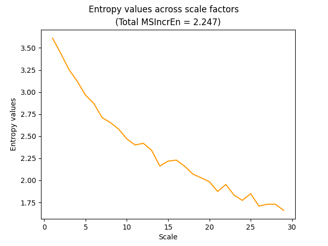
References

Liu, X., Jiang, A., Xu, N., & Xue, J. (2016). Increment entropy as a measure of complexity for time series. Entropy, 18(1), 22.
Liu, X., Jiang, A., Xu, N., & Xue, J. (2016). Correction on Liu, X.; Jiang, A.; Xu, N.; Xue, J. Increment Entropy as a Measure of Complexity for Time Series. Entropy 2016, 18, 22. Entropy, 18(4), 133.
Liu, X., Wang, X., Zhou, X., & Jiang, A. (2018). Appropriate use of the increment entropy for electrophysiological time series. Computers in Biology and Medicine, 95, 13-23.

entropy_slope()#

entropy_slope(signal, dimension=3, thresholds=[0.1, 45], **kwargs)[source]#

Slope Entropy (SlopEn)

Slope Entropy (SlopEn) uses an alphabet of three symbols, 0, 1, and 2, with positive (+) and negative versions (-) of the last two. Each symbol covers a range of slopes for the segment joining two consecutive samples of the input data, and the Shannon entropy of the relative frequency of each pattern is computed.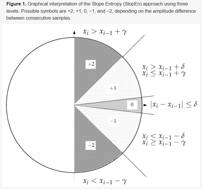

Parameters:

signal (Union[list, np.array, pd.Series]) – The signal (i.e., a time series) in the form of a vector of values.
dimension (int) – Embedding Dimension (m, sometimes referred to as d or order). See complexity_dimension() to estimate the optimal value for this parameter.
thresholds (list) – Angular thresholds (called levels). A list of monotonically increasing values in the range [0, 90] degrees.
**kwargs (optional) – Other keyword arguments, such as the logarithmic base to use for entropy_shannon().

Returns:

slopen (float) – Slope Entropy of the signal.
info (dict) – A dictionary containing additional information regarding the parameters used.

See also

entropy_shannon

Examples

In [1]: import neurokit2 as nk

# Simulate a Signal
In [2]: signal = nk.signal_simulate(duration=2, sampling_rate=200, frequency=[5, 6], noise=0.5)

# Compute Slope Entropy
In [3]: slopen, info = nk.entropy_slope(signal, dimension=3, thresholds=[0.1, 45])

In [4]: slopen
Out[4]: 3.8373480348752422

In [5]: slopen, info = nk.entropy_slope(signal, dimension=3, thresholds=[5, 45, 60, 90])

In [6]: slopen
Out[6]: 4.949755313900915

# Compute Multiscale Slope Entropy (MSSlopEn)
In [7]: msslopen, info = nk.entropy_multiscale(signal, method="MSSlopEn", show=True)

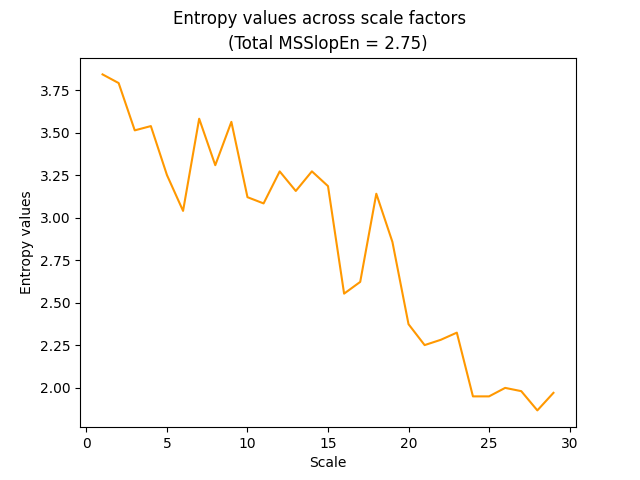
References

Cuesta-Frau, D. (2019). Slope entropy: A new time series complexity estimator based on both symbolic patterns and amplitude information. Entropy, 21(12), 1167.

entropy_symbolicdynamic()#

entropy_symbolicdynamic(signal, dimension=3, symbolize='MEP', c=6, **kwargs)[source]#

Symbolic Dynamic Entropy (SyDyEn) and its Multiscale variants (MSSyDyEn)

Symbolic Dynamic Entropy (SyDyEn) combines the merits of symbolic dynamic and information theory.

Parameters:

signal (Union[list, np.array, pd.Series]) – The signal (i.e., a time series) in the form of a vector of values.
dimension (int) – Embedding Dimension (m, sometimes referred to as d or order). See complexity_dimension() to estimate the optimal value for this parameter.
symbolize (str) – Method to convert a continuous signal input into a symbolic (discrete) signal. Can be one of "MEP" (default), "NCDF", "linear", "uniform", "kmeans", "equal", or others. See complexity_symbolize() for details.
c (int) – Number of symbols c.
**kwargs (optional) – Other keyword arguments (currently not used).

Returns:

SyDyEn (float) – Symbolic Dynamic Entropy (SyDyEn) of the signal.
info (dict) – A dictionary containing additional information regarding the parameters used.

Examples

In [1]: import neurokit2 as nk

In [2]: signal = [2, -7, -12, 5, -1, 9, 14]

# Simulate a Signal
In [3]: signal = nk.signal_simulate(duration=2, sampling_rate=200, frequency=[5, 6], noise=0.5)

# Compute Symbolic Dynamic Entropy
In [4]: sydyen, info = nk.entropy_symbolicdynamic(signal, c=3, symbolize="MEP")

In [5]: sydyen
Out[5]: 3.7574850006370646

In [6]: sydyen, info = nk.entropy_symbolicdynamic(signal, c=3, symbolize="kmeans")

In [7]: sydyen
Out[7]: 3.431184579303421

# Compute Multiscale Symbolic Dynamic Entropy (MSSyDyEn)
In [8]: mssydyen, info = nk.entropy_multiscale(signal, method="MSSyDyEn", show=True)

# Compute Modified Multiscale Symbolic Dynamic Entropy (MMSyDyEn)
In [9]: mmsydyen, info = nk.entropy_multiscale(signal, method="MMSyDyEn", show=True)

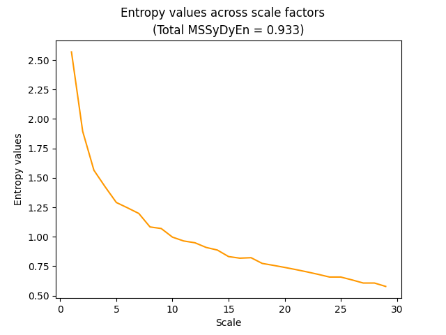
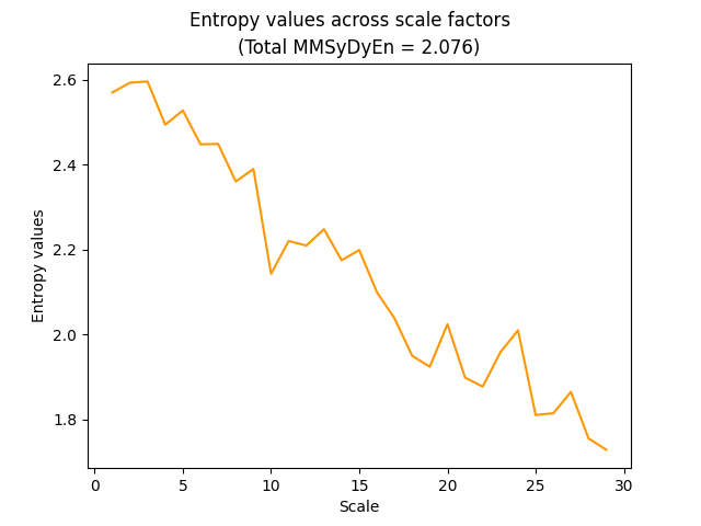
References

Matilla-García, M., Morales, I., Rodríguez, J. M., & Marín, M. R. (2021). Selection of embedding dimension and delay time in phase space reconstruction via symbolic dynamics. Entropy, 23(2), 221.
Li, Y., Yang, Y., Li, G., Xu, M., & Huang, W. (2017). A fault diagnosis scheme for planetary gearboxes using modified multi-scale symbolic dynamic entropy and mRMR feature selection. Mechanical Systems and Signal Processing, 91, 295-312.
Rajagopalan, V., & Ray, A. (2006). Symbolic time series analysis via wavelet-based partitioning. Signal processing, 86(11), 3309-3320.

entropy_dispersion()#

entropy_dispersion(signal, delay=1, dimension=3, c=6, symbolize='NCDF', fluctuation=False, rho=1, **kwargs)[source]#

Dispersion Entropy (DispEn)

The Dispersion Entropy (DispEn). Also returns the Reverse Dispersion Entropy (RDEn).

Parameters:

signal (Union[list, np.array, pd.Series]) – The signal (i.e., a time series) in the form of a vector of values.
delay (int) – Time delay (often denoted Tau $\tau$, sometimes referred to as lag) in samples. See complexity_delay() to estimate the optimal value for this parameter.
dimension (int) – Embedding Dimension (m, sometimes referred to as d or order). See complexity_dimension() to estimate the optimal value for this parameter.
c (int) – Number of symbols c. Rostaghi (2016) recommend in practice a c between 4 and 8.
symbolize (str) – Method to convert a continuous signal input into a symbolic (discrete) signal. Can be one of "NCDF" (default), "finesort", or others. See complexity_symbolize() for details.
fluctuation (bool) – Fluctuation-based Dispersion entropy.
rho (float) – Tuning parameter of “finesort”. Only when method="finesort".
**kwargs (optional) – Other keyword arguments (currently not used).

Returns:

DispEn (float) – Dispersion Entropy (DispEn) of the signal.
info (dict) – A dictionary containing additional information regarding the parameters used.

Examples

In [1]: import neurokit2 as nk

# Simulate a Signal
In [2]: signal = nk.signal_simulate(duration=2, sampling_rate=200, frequency=[5, 6], noise=0.5)

# Compute Dispersion Entropy (DispEn)
In [3]: dispen, info = nk.entropy_dispersion(signal, c=3)

In [4]: dispen
Out[4]: 1.3659519856214257

# Get Reverse Dispersion Entropy (RDEn)
In [5]: info["RDEn"]
Out[5]: 0.015269622173488236

# Fluctuation-based DispEn with "finesort"
In [6]: dispen, info = nk.entropy_dispersion(signal, c=3, symbolize="finesort", fluctuation=True)

In [7]: dispen
Out[7]: 1.3659519856214257

References

Rostaghi, M., & Azami, H. (2016). Dispersion entropy: A measure for time-series analysis. IEEE Signal Processing Letters, 23(5), 610-614.

entropy_ofentropy()#

entropy_ofentropy(signal, scale=10, bins=10, **kwargs)[source]#

Entropy of entropy (EnofEn)

Entropy of entropy (EnofEn or EoE) combines the features of MSE with an alternate measure of information, called superinformation, used in DNA sequencing.

Parameters:

signal (Union[list, np.array, pd.Series]) – The signal (i.e., a time series) in the form of a vector of values.
scale (int) – The size of the windows that the signal is divided into. Also referred to as Tau $\tau$, it represents the scale factor and corresponds to the amount of coarsegraining.
bins (int) – The number of equal-size bins to divide the signal’s range in.
**kwargs (optional) – Other keyword arguments, such as the logarithmic base to use for entropy_shannon().

Returns:

enofen (float) – The Entropy of entropy of the signal.
info (dict) – A dictionary containing additional information regarding the parameters used, such as the average entropy AvEn.

See also

entropy_shannon, entropy_multiscale

Examples

In [1]: import neurokit2 as nk

# Simulate a Signal
In [2]: signal = nk.signal_simulate(duration=2, sampling_rate=200, frequency=[5, 6], noise=0.5)

# EnofEn
In [3]: enofen, _ = nk.entropy_ofentropy(signal, scale=10, bins=10)

In [4]: enofen
Out[4]: 3.9428966084191095

References

Hsu, C. F., Wei, S. Y., Huang, H. P., Hsu, L., Chi, S., & Peng, C. K. (2017). Entropy of entropy: Measurement of dynamical complexity for biological systems. Entropy, 19(10), 550.

entropy_permutation()#

entropy_permutation(signal, delay=1, dimension=3, corrected=True, weighted=False, conditional=False, **kwargs)[source]#

Permutation Entropy (PEn), its Weighted (WPEn) and Conditional (CPEn) forms

Permutation Entropy (PEn) is a robust measure of the complexity of a dynamic system by capturing the order relations between values of a time series and extracting a probability distribution of the ordinal patterns (see Henry and Judge, 2019). Using ordinal descriptors increases robustness to large artifacts occurring with low frequencies. PEn is applicable for regular, chaotic, noisy, or real-world time series and has been employed in the context of EEG, ECG, and stock market time series.

Mathematically, it corresponds to the Shannon entropy after the signal has been made discrete by analyzing the permutations in the time-embedded space.

However, the main shortcoming of traditional PEn is that no information besides the order structure is retained when extracting the ordinal patterns, which leads to several possible issues (Fadlallah et al., 2013). The Weighted PEn was developed to address these limitations by incorporating significant information (regarding the amplitude) from the original time series into the ordinal patterns.

The Conditional Permutation Entropy (CPEn) was originally defined by Bandt & Pompe as Sorting Entropy, but recently gained in popularity as conditional through the work of Unakafov et al. (2014). It describes the average diversity of the ordinal patterns succeeding a given ordinal pattern (dimension+1 vs. dimension).

This function can be called either via entropy_permutation() or complexity_pe(). Moreover, variants can be directly accessed via complexity_wpe() and complexity_mspe().

Parameters:

signal (Union[list, np.array, pd.Series]) – The signal (i.e., a time series) in the form of a vector of values.
delay (int) – Time delay (often denoted Tau $\tau$, sometimes referred to as lag) in samples. See complexity_delay() to estimate the optimal value for this parameter.
dimension (int) – Embedding Dimension (m, sometimes referred to as d or order). See complexity_dimension() to estimate the optimal value for this parameter.
corrected (bool) – If True, divide by log2(factorial(m)) to normalize the entropy between 0 and 1. Otherwise, return the permutation entropy in bit.
weighted (bool) – If True, compute the weighted permutation entropy (WPE).
**kwargs – Optional arguments, such as a function to compute Entropy (nk.entropy_shannon() (default), nk.entropy_tsallis() or nk.entropy_reyni()).

Returns:

PEn (float) – Permutation Entropy
info (dict) – A dictionary containing additional information regarding the parameters used.

Examples

In [1]: signal = nk.signal_simulate(duration=2, sampling_rate=100, frequency=[5, 6], noise=0.5)

# Permutation Entropy (uncorrected)
In [2]: pen, info = nk.entropy_permutation(signal, corrected=False)

In [3]: pen
Out[3]: 2.5535541443514806

# Weighted Permutation Entropy (WPEn)
In [4]: wpen, info = nk.entropy_permutation(signal, weighted=True)

In [5]: wpen
Out[5]: 0.9867172080691854

# Conditional Permutation Entropy (CPEn)
In [6]: cpen, info = nk.entropy_permutation(signal, conditional=True)

In [7]: cpen
Out[7]: 0.4177834332353863

# Conditional Weighted Permutation Entropy (CWPEn)
In [8]: cwpen, info = nk.entropy_permutation(signal, weighted=True, conditional=True)

In [9]: cwpen
Out[9]: 0.40580048874793767

# Conditional Renyi Permutation Entropy (CRPEn)
In [10]: crpen, info = nk.entropy_permutation(signal, conditional=True, algorithm=nk.entropy_renyi, alpha=2)

In [11]: crpen
Out[11]: 0.2799671584220142

References

Henry, M., & Judge, G. (2019). Permutation entropy and information recovery in nonlinear dynamic economic time series. Econometrics, 7(1), 10.
Fadlallah, B., Chen, B., Keil, A., & Principe, J. (2013). Weighted-permutation entropy: A complexity measure for time series incorporating amplitude information. Physical Review E, 87 (2), 022911.
Zanin, M., Zunino, L., Rosso, O. A., & Papo, D. (2012). Permutation entropy and its main biomedical and econophysics applications: a review. Entropy, 14(8), 1553-1577.
Bandt, C., & Pompe, B. (2002). Permutation entropy: a natural complexity measure for time series. Physical review letters, 88(17), 174102.
Unakafov, A. M., & Keller, K. (2014). Conditional entropy of ordinal patterns. Physica D: Nonlinear Phenomena, 269, 94-102.

entropy_bubble()#

entropy_bubble(signal, delay=1, dimension=3, alpha=2, **kwargs)[source]#

Bubble Entropy (BubblEn)

Introduced by Manis et al. (2017) with the goal of being independent of parameters such as Tolerance and Dimension. Bubble Entropy is based on permutation entropy, but uses the bubble sort algorithm for the ordering procedure instead of the number of swaps performed for each vector.

Parameters:

signal (Union[list, np.array, pd.Series]) – The signal (i.e., a time series) in the form of a vector of values.
delay (int) – Time delay (often denoted Tau $\tau$, sometimes referred to as lag) in samples. See complexity_delay() to estimate the optimal value for this parameter.
dimension (int) – Embedding Dimension (m, sometimes referred to as d or order). See complexity_dimension() to estimate the optimal value for this parameter.
tolerance (float) – Tolerance (often denoted as r), distance to consider two data points as similar. If "sd" (default), will be set to $0.2 * SD_{signal}$. See complexity_tolerance() to estimate the optimal value for this parameter.
alpha (float) – The alpha $\alpha$ parameter (default to 1) for Rényi entropy).
**kwargs (optional) – Other arguments.

Returns:

BubbEn (float) – The Bubble Entropy.
info (dict) – A dictionary containing additional information regarding the parameters used to compute sample entropy.

Examples

In [1]: import neurokit2 as nk

In [2]: signal = nk.signal_simulate(duration=2, frequency=5)

In [3]: BubbEn, info = nk.entropy_bubble(signal)

In [4]: BubbEn
Out[4]: 0.07799253889312076

References

Manis, G., Aktaruzzaman, M. D., & Sassi, R. (2017). Bubble entropy: An entropy almost free of parameters. IEEE Transactions on Biomedical Engineering, 64(11), 2711-2718.

entropy_range()#

entropy_range(signal, dimension=3, delay=1, tolerance='sd', approximate=False, **kwargs)[source]#

Range Entropy (RangEn)

Introduced by Omidvarnia et al. (2018), Range Entropy (RangEn or RangeEn) refers to a modified form of SampEn (or ApEn).

Both ApEn and SampEn compute the logarithmic likelihood that runs of patterns that are close remain close on the next incremental comparisons, of which this closeness is estimated by the Chebyshev distance. Range Entropy uses instead a normalized “range distance”, resulting in modified forms of ApEn and SampEn, RangEn (A) (mApEn) and RangEn (B) (mSampEn).

However, the RangEn (A), based on ApEn, often yields undefined entropies (i.e., NaN or Inf). As such, using RangEn (B) is recommended instead.

RangEn is described as more robust to nonstationary signal changes, and has a more linear relationship with the Hurst exponent (compared to ApEn and SampEn), and has no need for signal amplitude correction.

Note that the corrected version of ApEn (cApEn) can be computed by setting corrected=True.

Parameters:

signal (Union[list, np.array, pd.Series]) – The signal (i.e., a time series) in the form of a vector of values.
delay (int) – Time delay (often denoted Tau $\tau$, sometimes referred to as lag) in samples. See complexity_delay() to estimate the optimal value for this parameter.
dimension (int) – Embedding Dimension (m, sometimes referred to as d or order). See complexity_dimension() to estimate the optimal value for this parameter.
tolerance (float) – Tolerance (often denoted as r), distance to consider two data points as similar. If "sd" (default), will be set to $0.2 * SD_{signal}$. See complexity_tolerance() to estimate the optimal value for this parameter.
approximate (bool) – The entropy algorithm to use. If False (default), will use sample entropy and return mSampEn (RangEn B). If True, will use approximate entropy and return mApEn (RangEn A).
**kwargs – Other arguments.

See also

entropy_approximate, entropy_sample

Returns:

RangEn (float) – Range Entropy. If undefined conditional probabilities are detected (logarithm of sum of conditional probabilities is ln(0)), np.inf will be returned, meaning it fails to retrieve ‘accurate’ regularity information. This tends to happen for short data segments, increasing tolerance levels might help avoid this.
info (dict) – A dictionary containing additional information regarding the parameters used.

Examples

In [1]: import neurokit2 as nk

In [2]: signal = nk.signal_simulate(duration=2, sampling_rate=100, frequency=[5, 6])

# Range Entropy B (mSampEn)
In [3]: RangEnB, info = nk.entropy_range(signal, approximate=False)

In [4]: RangEnB
Out[4]: 1.0882982278736182

# Range Entropy A (mApEn)
In [5]: RangEnA, info = nk.entropy_range(signal, approximate=True)

In [6]: RangEnA
Out[6]: 1.0749312293123292

# Range Entropy A (corrected)
In [7]: RangEnAc, info = nk.entropy_range(signal, approximate=True, corrected=True)

In [8]: RangEnAc
Out[8]: 1.1153142451616476

References

Omidvarnia, A., Mesbah, M., Pedersen, M., & Jackson, G. (2018). Range entropy: A bridge between signal complexity and self-similarity. Entropy, 20(12), 962.

entropy_fuzzy()#

entropy_fuzzy(signal, delay=1, dimension=2, tolerance='sd', approximate=False, **kwargs)[source]#

Fuzzy Entropy (FuzzyEn)

Fuzzy entropy (FuzzyEn) of a signal stems from the combination between information theory and fuzzy set theory (Zadeh, 1965). A fuzzy set is a set containing elements with varying degrees of membership.

This function can be called either via entropy_fuzzy() or complexity_fuzzyen(), or complexity_fuzzyapen() for its approximate version. Note that the fuzzy corrected approximate entropy (cApEn) can also be computed via setting corrected=True (see examples).

Parameters:

signal (Union[list, np.array, pd.Series]) – The signal (i.e., a time series) in the form of a vector of values.
delay (int) – Time delay (often denoted Tau $\tau$, sometimes referred to as lag) in samples. See complexity_delay() to estimate the optimal value for this parameter.
dimension (int) – Embedding Dimension (m, sometimes referred to as d or order). See complexity_dimension() to estimate the optimal value for this parameter.
tolerance (float) – Tolerance (often denoted as r), distance to consider two data points as similar. If "sd" (default), will be set to $0.2 * SD_{signal}$. See complexity_tolerance() to estimate the optimal value for this parameter.
approximate (bool) – If True, will compute the fuzzy approximate entropy (FuzzyApEn).
**kwargs – Other arguments.

Returns:

fuzzyen (float) – The fuzzy entropy of the single time series.
info (dict) – A dictionary containing additional information regarding the parameters used to compute fuzzy entropy.

See also

entropy_sample

Examples

..ipython:: python

import neurokit2 as nk

signal = nk.signal_simulate(duration=2, frequency=5)

fuzzyen, parameters = nk.entropy_fuzzy(signal) fuzzyen

fuzzyapen, parameters = nk.entropy_fuzzy(signal, approximate=True) fuzzyapen

fuzzycapen, parameters = nk.entropy_fuzzy(signal, approximate=True, corrected=True) fuzzycapen

References

Ishikawa, A., & Mieno, H. (1979). The fuzzy entropy concept and its application. Fuzzy Sets and systems, 2(2), 113-123.
Zadeh, L. A. (1996). Fuzzy sets. In Fuzzy sets, fuzzy logic, and fuzzy systems: selected papers by Lotfi A Zadeh (pp. 394-432).

entropy_multiscale()#

entropy_multiscale(signal, scale='default', dimension=3, tolerance='sd', method='MSEn', show=False, **kwargs)[source]#

Multiscale entropy (MSEn) and its Composite (CMSEn), Refined (RCMSEn) or fuzzy versions

One of the limitation of SampEn is that it characterizes complexity strictly on the time scale defined by the sampling procedure (via the delay argument). To address this, Costa et al. (2002) proposed the multiscale entropy (MSEn), which computes sample entropies at multiple scales.

The conventional MSEn algorithm consists of two steps:

A coarse-graining procedure is used to represent the signal at different time scales.
Sample entropy (or other function) is used to quantify the regularity of a coarse-grained time series at each time scale factor.

However, in the traditional coarse-graining procedure, the larger the scale factor is, the shorter the coarse-grained time series is. As such, the variance of the entropy of the coarse-grained series estimated by SampEn increases as the time scale factor increases, making it problematic for shorter signals.

CMSEn: In order to reduce the variance of estimated entropy values at large scales, Wu et al. (2013) introduced the Composite Multiscale Entropy algorithm, which computes multiple coarse-grained series for each scale factor (via the time-shift method for coarse-graining).
RCMSEn: Wu et al. (2014) further Refined their CMSEn by averaging not the entropy values of each subcoarsed vector, but its components at a lower level.
MMSEn: Wu et al. (2013) also introduced the Modified Multiscale Entropy algorithm, which is based on rolling-average coarse-graining.
IMSEn: Liu et al. (2012) introduced an adaptive-resampling procedure to resample the coarse-grained series. We implement a generalization of this via interpolation that can be referred to as Interpolated Multiscale Entropy.

Warning

Interpolated Multiscale variants don’t work as expected. Help is needed to fix this procedure.

Their Fuzzy version can be obtained by setting fuzzy=True.

This function can be called either via entropy_multiscale() or complexity_mse(). Moreover, variants can be directly accessed via complexity_cmse(), complexity_rcmse()`, complexity_fuzzymse(), complexity_fuzzycmse() and complexity_fuzzyrcmse().

Parameters:

signal (Union[list, np.array, pd.Series]) – The signal (i.e., a time series) in the form of a vector of values. or dataframe.
scale (str or int or list) – A list of scale factors used for coarse graining the time series. If ‘default’, will use range(len(signal) / (dimension + 10)) (see discussion here). If ‘max’, will use all scales until half the length of the signal. If an integer, will create a range until the specified int. See complexity_coarsegraining() for details.
dimension (int) – Embedding Dimension (m, sometimes referred to as d or order). See complexity_dimension() to estimate the optimal value for this parameter.
tolerance (float) – Tolerance (often denoted as r), distance to consider two data points as similar. If "sd" (default), will be set to $0.2 * SD_{signal}$. See complexity_tolerance() to estimate the optimal value for this parameter.
method (str) – What version of multiscale entropy to compute. Can be one of "MSEn", "CMSEn", "RCMSEn", "MMSEn", "IMSEn", "MSApEn", "MSPEn", "CMSPEn", "MMSPEn", "IMSPEn", "MSWPEn", "CMSWPEn", "MMSWPEn", "IMSWPEn" (case sensitive).
show (bool) – Show the entropy values for each scale factor.
**kwargs – Optional arguments.

Returns:

float – The point-estimate of multiscale entropy (MSEn) of the single time series corresponding to the area under the MSEn values curve, which is essentially the sum of sample entropy values over the range of scale factors.
dict – A dictionary containing additional information regarding the parameters used to compute multiscale entropy. The entropy values corresponding to each "Scale" factor are stored under the "Value" key.

Examples

MSEn (basic coarse-graining)

In [1]: import neurokit2 as nk

In [2]: signal = nk.signal_simulate(duration=2, frequency=[5, 12, 40])

In [3]: msen, info = nk.entropy_multiscale(signal, show=True)

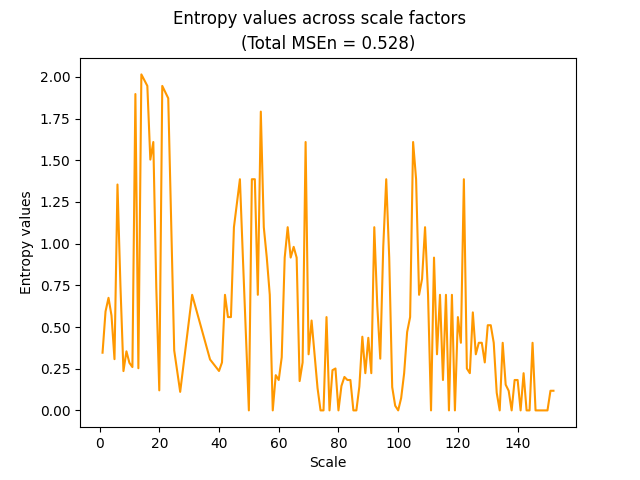
CMSEn (time-shifted coarse-graining)

In [4]: cmsen, info = nk.entropy_multiscale(signal, method="CMSEn", show=True)

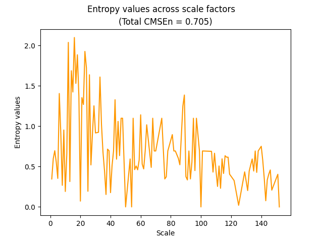
RCMSEn (refined composite MSEn)

In [5]: rcmsen, info = nk.entropy_multiscale(signal, method="RCMSEn", show=True)

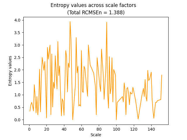
MMSEn (rolling-window coarse-graining)

In [6]: mmsen, info = nk.entropy_multiscale(signal, method="MMSEn", show=True)

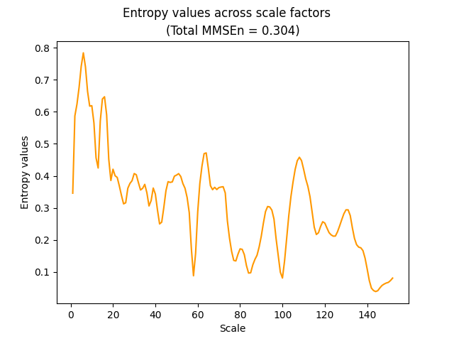
IMSEn (interpolated coarse-graining)

In [7]: imsen, info = nk.entropy_multiscale(signal, method="IMSEn", show=True)

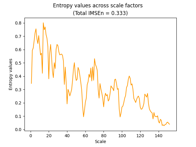
MSApEn (based on ApEn instead of SampEn)

In [8]: msapen, info = nk.entropy_multiscale(signal, method="MSApEn", show=True)

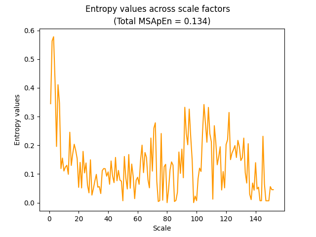
MSPEn (based on PEn), CMSPEn, MMSPEn and IMSPEn

In [9]: mspen, info = nk.entropy_multiscale(signal, method="MSPEn", show=True)

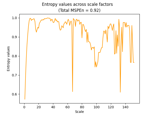
In [10]: cmspen, info = nk.entropy_multiscale(signal, method="CMSPEn")

In [11]: cmspen
Out[11]: 0.9270529263870483

In [12]: mmspen, info = nk.entropy_multiscale(signal, method="MMSPEn")

In [13]: mmspen
Out[13]: 0.953782723664592

In [14]: imspen, info = nk.entropy_multiscale(signal, method="IMSPEn")

In [15]: imspen
Out[15]: 0.954390411042964

MSWPEn (based on WPEn), CMSWPEn, MMSWPEn and IMSWPEn

In [16]: mswpen, info = nk.entropy_multiscale(signal, method="MSWPEn")

In [17]: cmswpen, info = nk.entropy_multiscale(signal, method="CMSWPEn")

In [18]: mmswpen, info = nk.entropy_multiscale(signal, method="MMSWPEn")

In [19]: imswpen, info = nk.entropy_multiscale(signal, method="IMSWPEn")

FuzzyMSEn, FuzzyCMSEn and FuzzyRCMSEn

In [20]: fuzzymsen, info = nk.entropy_multiscale(signal, method="MSEn", fuzzy=True, show=True)

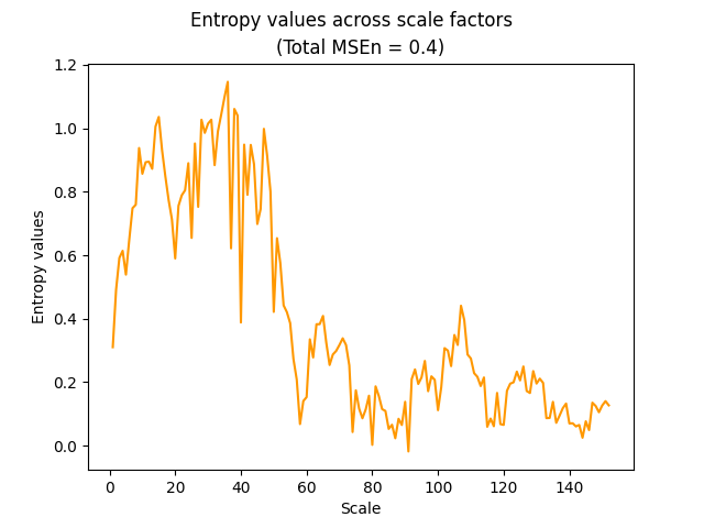
In [21]: fuzzycmsen, info = nk.entropy_multiscale(signal, method="CMSEn", fuzzy=True)

In [22]: fuzzycmsen
Out[22]: 1.0155636506693684

In [23]: fuzzyrcmsen, info = nk.entropy_multiscale(signal, method="RCMSEn", fuzzy=True)

In [24]: fuzzycmsen
Out[24]: 1.0155636506693684

References

Costa, M., Goldberger, A. L., & Peng, C. K. (2002). Multiscale entropy analysis of complex physiologic time series. Physical review letters, 89(6), 068102.
Costa, M., Goldberger, A. L., & Peng, C. K. (2005). Multiscale entropy analysis of biological signals. Physical review E, 71(2), 021906.
Wu, S. D., Wu, C. W., Lee, K. Y., & Lin, S. G. (2013). Modified multiscale entropy for short-term time series analysis. Physica A: Statistical Mechanics and its Applications, 392 (23), 5865-5873.
Wu, S. D., Wu, C. W., Lin, S. G., Wang, C. C., & Lee, K. Y. (2013). Time series analysis using composite multiscale entropy. Entropy, 15(3), 1069-1084.
Wu, S. D., Wu, C. W., Lin, S. G., Lee, K. Y., & Peng, C. K. (2014). Analysis of complex time series using refined composite multiscale entropy. Physics Letters A, 378(20), 1369-1374.
Gow, B. J., Peng, C. K., Wayne, P. M., & Ahn, A. C. (2015). Multiscale entropy analysis of center-of-pressure dynamics in human postural control: methodological considerations. Entropy, 17(12), 7926-7947.
Norris, P. R., Anderson, S. M., Jenkins, J. M., Williams, A. E., & Morris Jr, J. A. (2008). Heart rate multiscale entropy at three hours predicts hospital mortality in 3,154 trauma patients. Shock, 30(1), 17-22.
Liu, Q., Wei, Q., Fan, S. Z., Lu, C. W., Lin, T. Y., Abbod, M. F., & Shieh, J. S. (2012). Adaptive computation of multiscale entropy and its application in EEG signals for monitoring depth of anesthesia during surgery. Entropy, 14(6), 978-992.

entropy_hierarchical()#

entropy_hierarchical(signal, scale='default', dimension=2, tolerance='sd', show=False, **kwargs)[source]#

Hierarchical Entropy (HEn)

Hierarchical Entropy (HEn) can be viewed as a generalization of the multiscale decomposition used in multiscale entropy, and the Haar wavelet decomposition since it generate subtrees of the hierarchical tree. It preserves the strength of the multiscale decomposition with additional components of higher frequency in different scales. The hierarchical decomposition, unlike the wavelet decomposition, contains redundant components, which makes it sensitive to the dynamical richness of the time series.

Parameters:

signal (Union[list, np.array, pd.Series]) – The signal (i.e., a time series) in the form of a vector of values.
scale (int) – The maximum scale factor. Can only be a number of “default”. Though it behaves a bit differently here, see complexity_multiscale() for details.
dimension (int) – Embedding Dimension (m, sometimes referred to as d or order). See complexity_dimension() to estimate the optimal value for this parameter.
method (str) – Method for symbolic sequence partitioning. Can be one of "MEP" (default), "linear", "uniform", "kmeans".
**kwargs (optional) – Other keyword arguments (currently not used).

Returns:

SyDyEn (float) – Symbolic Dynamic Entropy (SyDyEn) of the signal.
info (dict) – A dictionary containing additional information regarding the parameters used.

See also

entropy_shannon, entropy_multiscale

Examples

In [1]: import neurokit2 as nk

# Simulate a Signal
In [2]: signal = nk.signal_simulate(duration=5, frequency=[97, 98, 100], noise=0.05)

# Compute Hierarchical Entropy (HEn)
In [3]: hen, info = nk.entropy_hierarchical(signal, show=True, scale=5, dimension=3)

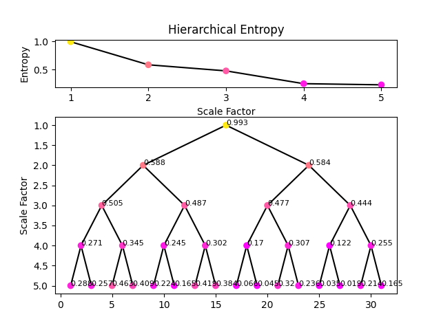
References

Jiang, Y., Peng, C. K., & Xu, Y. (2011). Hierarchical entropy analysis for biological signals. Journal of Computational and Applied Mathematics, 236(5), 728-742.
Li, W., Shen, X., & Li, Y. (2019). A comparative study of multiscale sample entropy and hierarchical entropy and its application in feature extraction for ship-radiated noise. Entropy, 21(8), 793.

Other indices#

fisher_information()#

fisher_information(signal, delay=1, dimension=2)[source]#

Fisher Information (FI)

The Fisher information was introduced by R. A. Fisher in 1925, as a measure of “intrinsic accuracy” in statistical estimation theory. It is central to many statistical fields far beyond that of complexity theory. It measures the amount of information that an observable random variable carries about an unknown parameter. In complexity analysis, the amount of information that a system carries “about itself” is measured. Similarly to SVDEn, it is based on the Singular Value Decomposition (SVD) of the time-delay embedded signal. The value of FI is usually anti-correlated with other measures of complexity (the more information a system withholds about itself, and the more predictable and thus, less complex it is).

Parameters:

signal (Union[list, np.array, pd.Series]) – The signal (i.e., a time series) in the form of a vector of values.
delay (int) – Time delay (often denoted Tau $\tau$, sometimes referred to as lag) in samples. See complexity_delay() to estimate the optimal value for this parameter.
dimension (int) – Embedding Dimension (m, sometimes referred to as d or order). See complexity_dimension() to estimate the optimal value for this parameter.

Returns:

fi (float) – The computed fisher information measure.
info (dict) – A dictionary containing additional information regarding the parameters used to compute fisher information.

Examples

In [1]: import neurokit2 as nk

In [2]: signal = nk.signal_simulate(duration=2, frequency=5)

In [3]: fi, info = nk.fisher_information(signal, delay=10, dimension=3)

In [4]: fi
Out[4]: 0.6424727558784687

fishershannon_information()#

fishershannon_information(signal, **kwargs)[source]#

Fisher-Shannon Information (FSI)

The Shannon Entropy Power is closely related to another index, the Fisher Information Measure (FIM). Their combination results in the Fisher-Shannon Information index.

Warning

We are not sure at all about the correct implementation of this function. Please consider helping us by double-checking the code against the formulas in the references.

Parameters:

signal (Union[list, np.array, pd.Series]) – The signal (i.e., a time series) in the form of a vector of values.
**kwargs – Other arguments to be passed to density_bandwidth().

Returns:

fsi (float) – The computed FSI.
info (dict) – A dictionary containing additional information regarding the parameters used.

See also

entropy_power

Examples

In [1]: import neurokit2 as nk

In [2]: signal = nk.signal_simulate(duration=10, frequency=[10, 12], noise=0.1)

In [3]: fsi, info = nk.fishershannon_information(signal, method=0.01)

In [4]: fsi
Out[4]: 0.00028474116321757886

References

Guignard, F., Laib, M., Amato, F., & Kanevski, M. (2020). Advanced analysis of temporal data using Fisher-Shannon information: theoretical development and application in geosciences. Frontiers in Earth Science, 8, 255.
Vignat, C., & Bercher, J. F. (2003). Analysis of signals in the Fisher-Shannon information plane. Physics Letters A, 312(1-2), 27-33.

mutual_information()#

mutual_information(x, y, method='varoquaux', bins='default', **kwargs)[source]#

Mutual Information (MI)

Computes the mutual information (MI) between two vectors from a joint histogram. The mutual information of two variables is a measure of the mutual dependence between them. More specifically, it quantifies the “amount of information” obtained about one variable by observing the other variable.

Different methods are available:

nolitsa: Standard mutual information (a bit faster than the "sklearn" method).
varoquaux: Applies a Gaussian filter on the joint-histogram. The smoothing amount can be modulated via the sigma argument (by default, sigma=1).
knn: Non-parametric (i.e., not based on binning) estimation via nearest neighbors. Additional parameters includes k (by default, k=3), the number of nearest neighbors to use.
max: Maximum Mutual Information coefficient, i.e., the MI is maximal given a certain combination of number of bins.

Parameters:

x (Union[list, np.array, pd.Series]) – A vector of values.
y (Union[list, np.array, pd.Series]) – A vector of values.
method (str) – The method to use.
bins (int) – Number of bins to use while creating the histogram. Only used for "nolitsa" and "varoquaux". If "default", the number of bins is estimated following Hacine-Gharbi (2018).
**kwargs – Additional keyword arguments to pass to the chosen method.

Returns:

float – The computed similarity measure.

See also

information_fisher

Examples

Example 1: Simple case

In [1]: import neurokit2 as nk

In [2]: x = [3, 3, 5, 1, 6, 3, 2, 8, 1, 2, 3, 5, 4, 0, 2]

In [3]: y = [5, 3, 1, 3, 4, 5, 6, 4, 1, 3, 4, 6, 2, 1, 3]

In [4]: nk.mutual_information(x, y, method="varoquaux")
Out[4]: 0.0001470209869369743

In [5]: nk.mutual_information(x, y, method="nolitsa")
Out[5]: 0.22002600168808772

In [6]: nk.mutual_information(x, y, method="knn")
Out[6]: 1.2435788908307561

In [7]: nk.mutual_information(x, y, method="max")
Out[7]: 0.19200837690707584

Example 2: Method comparison

In [8]: import numpy as np

In [9]: import pandas as pd

In [10]: x = np.random.normal(size=400)

In [11]: y = x**2

In [12]: data = pd.DataFrame()

In [13]: for level in np.linspace(0.01, 3, 200):
   ....:     noise = np.random.normal(scale=level, size=400)
   ....:     rez = pd.DataFrame({"Noise": [level]})
   ....:     rez["MI1"] = nk.mutual_information(x, y + noise, method="varoquaux", sigma=1)
   ....:     rez["MI2"] = nk.mutual_information(x, y + noise, method="varoquaux", sigma=0)
   ....:     rez["MI3"] = nk.mutual_information(x, y + noise, method="nolitsa")
   ....:     rez["MI4"] = nk.mutual_information(x, y + noise, method="knn")
   ....:     rez["MI5"] = nk.mutual_information(x, y + noise, method="max")
   ....:     data = pd.concat([data, rez], axis=0)
   ....: 

In [14]: data["MI1"] = nk.rescale(data["MI1"])

In [15]: data["MI2"] = nk.rescale(data["MI2"])

In [16]: data["MI3"] = nk.rescale(data["MI3"])

In [17]: data["MI4"] = nk.rescale(data["MI4"])

In [18]: data["MI5"] = nk.rescale(data["MI5"])

In [19]: data.plot(x="Noise", y=["MI1", "MI2", "MI3", "MI4", "MI5"], kind="line")
Out[19]: <Axes: xlabel='Noise'>

# Computation time
# x = np.random.normal(size=10000)
# %timeit nk.mutual_information(x, x**2, method="varoquaux")
# %timeit nk.mutual_information(x, x**2, method="nolitsa")
# %timeit nk.mutual_information(x, x**2, method="sklearn")
# %timeit nk.mutual_information(x, x**2, method="knn", k=2)
# %timeit nk.mutual_information(x, x**2, method="knn", k=5)
# %timeit nk.mutual_information(x, x**2, method="max")

References

Studholme, C., Hawkes, D. J., & Hill, D. L. (1998, June). Normalized entropy measure for multimodality image alignment. In Medical imaging 1998: image processing (Vol. 3338, pp. 132-143). SPIE.
Hacine-Gharbi, A., & Ravier, P. (2018). A binning formula of bi-histogram for joint entropy estimation using mean square error minimization. Pattern Recognition Letters, 101, 21-28.

complexity_hjorth()#

complexity_hjorth(signal)[source]#

Hjorth’s Complexity and Parameters

Hjorth Parameters are indicators of statistical properties initially introduced by Hjorth (1970) to describe the general characteristics of an EEG trace in a few quantitative terms, but which can applied to any time series. The parameters are activity, mobility, and complexity. NeuroKit returns complexity directly in the output tuple, but the other parameters can be found in the dictionary.

The activity parameter is simply the variance of the signal, which corresponds to the mean power of a signal (if its mean is 0).

\[Activity = \sigma_{signal}^2\]
The mobility parameter represents the mean frequency or the proportion of standard deviation of the power spectrum. This is defined as the square root of variance of the first derivative of the signal divided by the variance of the signal.

\[Mobility = \frac{\sigma_{dd}/ \sigma_{d}}{Complexity}\]
The complexity parameter gives an estimate of the bandwidth of the signal, which indicates the similarity of the shape of the signal to a pure sine wave (for which the value converges to 1). In other words, it is a measure of the “excessive details” with reference to the “softest” possible curve shape. The Complexity parameter is defined as the ratio of the mobility of the first derivative of the signal to the mobility of the signal.

\[Complexity = \sigma_{d}/ \sigma_{signal}\]

$d$ and $dd$ represent the first and second derivatives of the signal, respectively.

Hjorth (1970) illustrated the parameters as follows:

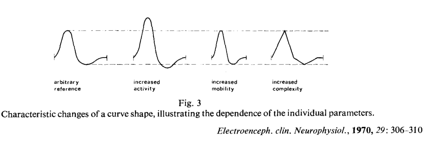
See also

fractal_petrosian

Parameters:

signal (Union[list, np.array, pd.Series]) – The signal (i.e., a time series) in the form of a vector of values.

Returns:

hjorth (float) – Hjorth’s Complexity.
info (dict) – A dictionary containing the additional Hjorth parameters, such as "Mobility" and "Activity".

Examples

In [1]: import neurokit2 as nk

# Simulate a signal with duration os 2s
In [2]: signal = nk.signal_simulate(duration=2, frequency=5)

# Compute Hjorth's Complexity
In [3]: complexity, info = nk.complexity_hjorth(signal)

In [4]: complexity
Out[4]: 1.0010008861067599

In [5]: info
Out[5]: {'Mobility': 0.03140677206992582, 'Activity': 0.125}

References

Hjorth, B (1970) EEG Analysis Based on Time Domain Properties. Electroencephalography and Clinical Neurophysiology, 29, 306-310.

complexity_decorrelation()#

complexity_decorrelation(signal, show=False)[source]#

Decorrelation Time (DT)

The decorrelation time (DT) is defined as the time (in samples) of the first zero crossing of the autocorrelation sequence. A shorter decorrelation time corresponds to a less correlated signal. For instance, a drop in the decorrelation time of EEG has been observed prior to seizures, related to a decrease in the low frequency power (Mormann et al., 2005).

Parameters:

signal (Union[list, np.array, pd.Series]) – The signal (i.e., a time series) in the form of a vector of values.
show (bool) – If True, will return a plot of the autocorrelation.

Returns:

float – Decorrelation Time (DT)
dict – A dictionary containing additional information (currently empty, but returned nonetheless for consistency with other functions).

See also

signal_autocor

Examples

In [1]: import neurokit2 as nk

# Simulate a signal
In [2]: signal = nk.signal_simulate(duration=5, sampling_rate=100, frequency=[5, 6], noise=0.5)

# Compute DT
In [3]: dt, _ = nk.complexity_decorrelation(signal, show=True)

In [4]: dt
Out[4]: 5

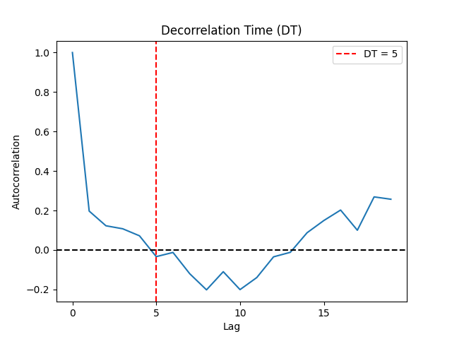
References

Mormann, F., Kreuz, T., Rieke, C., Andrzejak, R. G., Kraskov, A., David, P., … & Lehnertz, K. (2005). On the predictability of epileptic seizures. Clinical neurophysiology, 116(3), 569-587.
Teixeira, C. A., Direito, B., Feldwisch-Drentrup, H., Valderrama, M., Costa, R. P., Alvarado-Rojas, C., … & Dourado, A. (2011). EPILAB: A software package for studies on the prediction of epileptic seizures. Journal of Neuroscience Methods, 200(2), 257-271.

complexity_lempelziv()#

complexity_lempelziv(signal, delay=1, dimension=2, permutation=False, symbolize='mean', **kwargs)[source]#

Lempel-Ziv Complexity (LZC, PLZC and MSLZC)

Computes Lempel-Ziv Complexity (LZC) to quantify the regularity of the signal, by scanning symbolic sequences for new patterns, increasing the complexity count every time a new sequence is detected. Regular signals have a lower number of distinct patterns and thus have low LZC whereas irregular signals are characterized by a high LZC. While often being interpreted as a complexity measure, LZC was originally proposed to reflect randomness (Lempel and Ziv, 1976).

Permutation Lempel-Ziv Complexity (PLZC) combines LZC with permutation. A sequence of symbols is generated from the permutations observed in the tine-delay embedding, and LZC is computed over it.

Multiscale (Permutation) Lempel-Ziv Complexity (MSLZC or MSPLZC) combines permutation LZC with the multiscale approach. It first performs a coarse-graining procedure to the original time series.

Parameters:

signal (Union[list, np.array, pd.Series]) – The signal (i.e., a time series) in the form of a vector of values.
delay (int) – Time delay (often denoted Tau $\tau$, sometimes referred to as lag) in samples. See complexity_delay() to estimate the optimal value for this parameter. Only used when permutation=True.
dimension (int) – Embedding Dimension (m, sometimes referred to as d or order). See complexity_dimension() to estimate the optimal value for this parameter. Only used when permutation=True
permutation (bool) – If True, will return PLZC.
symbolize (str) – Only used when permutation=False. Method to convert a continuous signal input into a symbolic (discrete) signal. By default, assigns 0 and 1 to values below and above the mean. Can be None to skip the process (in case the input is already discrete). See complexity_symbolize() for details.
**kwargs – Other arguments to be passed to complexity_ordinalpatterns() (if permutation=True) or complexity_symbolize().

Returns:

lzc (float) – Lempel Ziv Complexity (LZC) of the signal.
info (dict) – A dictionary containing additional information regarding the parameters used to compute LZC.

Examples

In [1]: import neurokit2 as nk

In [2]: signal = nk.signal_simulate(duration=2, sampling_rate=200, frequency=[5, 6], noise=0.5)

# LZC
In [3]: lzc, info = nk.complexity_lempelziv(signal)

In [4]: lzc
Out[4]: 0.9940434618240934

# PLZC
In [5]: plzc, info = nk.complexity_lempelziv(signal, delay=1, dimension=3, permutation=True)

In [6]: plzc
Out[6]: 0.6631836579888775

# MSLZC
In [7]: mslzc, info = nk.entropy_multiscale(signal, method="LZC", show=True)

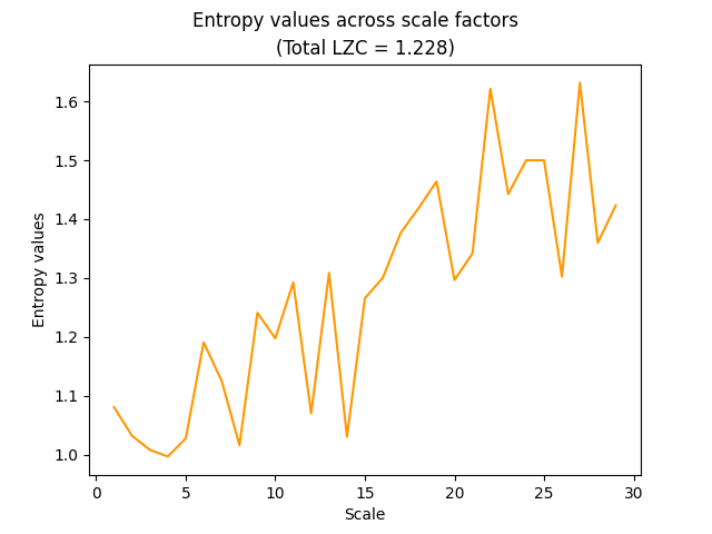
# MSPLZC
In [8]: msplzc, info = nk.entropy_multiscale(signal, method="LZC", permutation=True, show=True)

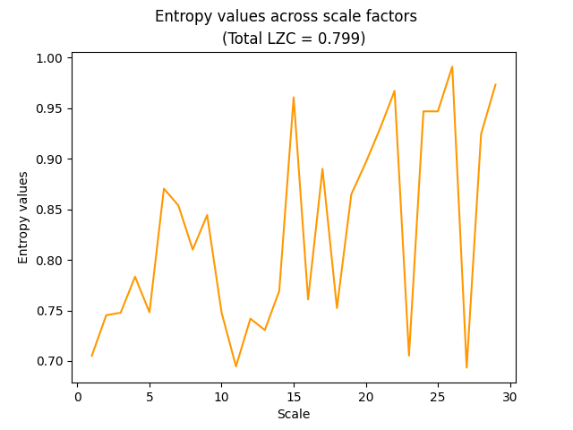
References

Lempel, A., & Ziv, J. (1976). On the complexity of finite sequences. IEEE Transactions on information theory, 22(1), 75-81.
Nagarajan, R. (2002). Quantifying physiological data with Lempel-Ziv complexity-certain issues. IEEE Transactions on Biomedical Engineering, 49(11), 1371-1373.
Kaspar, F., & Schuster, H. G. (1987). Easily calculable measure for the complexity of spatiotemporal patterns. Physical Review A, 36(2), 842.
Zhang, Y., Hao, J., Zhou, C., & Chang, K. (2009). Normalized Lempel-Ziv complexity and its application in bio-sequence analysis. Journal of mathematical chemistry, 46(4), 1203-1212.
Bai, Y., Liang, Z., & Li, X. (2015). A permutation Lempel-Ziv complexity measure for EEG analysis. Biomedical Signal Processing and Control, 19, 102-114.
Borowska, M. (2021). Multiscale Permutation Lempel-Ziv Complexity Measure for Biomedical Signal Analysis: Interpretation and Application to Focal EEG Signals. Entropy, 23(7), 832.

complexity_relativeroughness()#

complexity_relativeroughness(signal, **kwargs)[source]#

Relative Roughness (RR)

Relative Roughness is a ratio of local variance (autocovariance at lag-1) to global variance (autocovariance at lag-0) that can be used to classify different ‘noises’ (see Hasselman, 2019). It can also be used as an index to test for the applicability of fractal analysis (see Marmelat et al., 2012).

Parameters:

signal (Union[list, np.array, pd.Series]) – The signal (i.e., a time series) in the form of a vector of values.
**kwargs (optional) – Other arguments to be passed to nk.signal_autocor().

Returns:

rr (float) – The RR value.
info (dict) – A dictionary containing additional information regarding the parameters used to compute RR.

Examples

In [1]: import neurokit2 as nk

In [2]: signal = [1, 2, 3, 4, 5]

In [3]: rr, _ = nk.complexity_relativeroughness(signal)

In [4]: rr
Out[4]: 1.2

References

Marmelat, V., Torre, K., & Delignieres, D. (2012). Relative roughness: an index for testing the suitability of the monofractal model. Frontiers in Physiology, 3, 208.

complexity_lyapunov()#

complexity_lyapunov(signal, delay=1, dimension=2, method='rosenstein1993', separation='auto', **kwargs)[source]#

(Largest) Lyapunov Exponent (LLE)

Lyapunov exponents (LE) describe the rate of exponential separation (convergence or divergence) of nearby trajectories of a dynamical system. It is a measure of sensitive dependence on initial conditions, i.e. how quickly two nearby states diverge. A system can have multiple LEs, equal to the number of the dimensionality of the phase space, and the largest LE value, “LLE” is often used to determine the overall predictability of the dynamical system.

Different algorithms exist to estimate these indices:

Rosenstein et al.’s (1993) algorithm was designed for calculating LLEs from small datasets. The time series is first reconstructed using a delay-embedding method, and the closest neighbour of each vector is computed using the euclidean distance. These two neighbouring points are then tracked along their distance trajectories for a number of data points. The slope of the line using a least-squares fit of the mean log trajectory of the distances gives the final LLE.
Makowski is a custom modification of Rosenstein’s algorithm, using KDTree for more efficient nearest neighbors computation. Additionally, the LLE is computed as the slope up to the changepoint of divergence rate (the point where it flattens out), making it more robust to the length trajectory parameter.
Eckmann et al. (1986) computes LEs by first reconstructing the time series using a delay-embedding method, and obtains the tangent that maps to the reconstructed dynamics using a least-squares fit, where the LEs are deduced from the tangent maps.

Warning

The Eckman (1986) method currently does not work. Please help us fixing it by double checking the code, the paper and helping us figuring out what’s wrong. Overall, we would like to improve this function to return for instance all the exponents (Lyapunov spectrum), implement newer and faster methods (e.g., Balcerzak, 2018, 2020), etc. If you’re interested in helping out with this, please get in touch!

Parameters:

signal (Union[list, np.array, pd.Series]) – The signal (i.e., a time series) in the form of a vector of values.
delay (int) – Time delay (often denoted Tau $\tau$, sometimes referred to as lag) in samples. See complexity_delay() to estimate the optimal value for this parameter.
dimension (int) – Embedding Dimension (m, sometimes referred to as d or order). See complexity_dimension() to estimate the optimal value for this parameter. If method is "eckmann1986", larger values for dimension are recommended.
method (str) – The method that defines the algorithm for computing LE. Can be one of "rosenstein1993", "makowski", or "eckmann1986".
len_trajectory (int) – Applies when method is "rosenstein1993". The number of data points in which neighboring trajectories are followed.
matrix_dim (int) – Applies when method is "eckmann1986". Corresponds to the number of LEs to return.
min_neighbors (int, str) – Applies when method is "eckmann1986". Minimum number of neighbors. If "default", min(2 * matrix_dim, matrix_dim + 4) is used.
**kwargs (optional) – Other arguments to be passed to signal_psd() for calculating the minimum temporal separation of two neighbors.

Returns:

lle (float) – An estimate of the largest Lyapunov exponent (LLE) if method is "rosenstein1993", and an array of LEs if "eckmann1986".
info (dict) – A dictionary containing additional information regarding the parameters used to compute LLE.

Examples

In [1]: import neurokit2 as nk

In [2]: signal = nk.signal_simulate(duration=5, sampling_rate=100, frequency=[5, 8], noise=0.1)

# Rosenstein's method
In [3]: lle, info = nk.complexity_lyapunov(signal, method="rosenstein", show=True)

In [4]: lle
Out[4]: 0.06428137368015259

# Makowski's change-point method
In [5]: lle, info = nk.complexity_lyapunov(signal, method="makowski", show=True)

# Eckman's method is broken. Please help us fix-it!
# lle, info = nk.complexity_lyapunov(signal, dimension=2, method="eckmann1986")

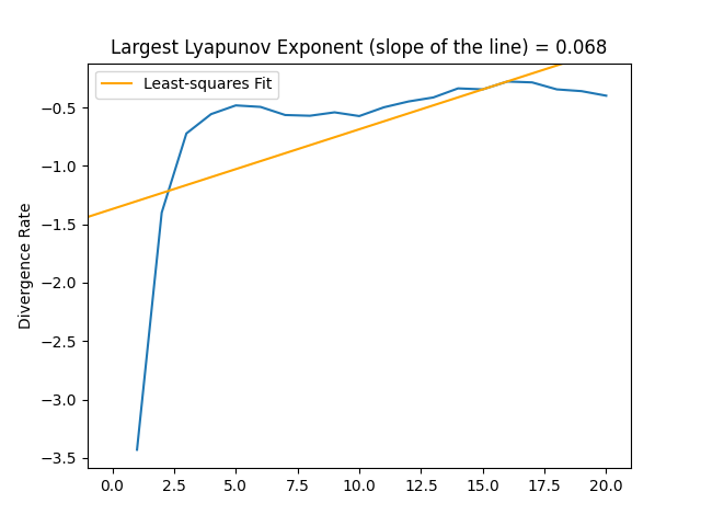
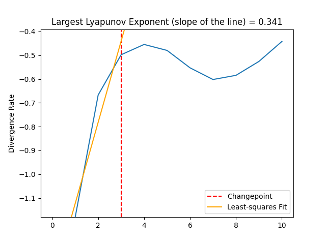
References

Rosenstein, M. T., Collins, J. J., & De Luca, C. J. (1993). A practical method for calculating largest Lyapunov exponents from small data sets. Physica D: Nonlinear Phenomena, 65(1-2), 117-134.
Eckmann, J. P., Kamphorst, S. O., Ruelle, D., & Ciliberto, S. (1986). Liapunov exponents from time series. Physical Review A, 34(6), 4971.

complexity_rqa()#

complexity_rqa(signal, dimension=3, delay=1, tolerance='sd', min_linelength=2, method='python', show=False)[source]#

Recurrence Quantification Analysis (RQA)

A recurrence plot is based on a time-delay embedding representation of a signal and is a 2D depiction of when a system revisits a state that is has been in the past.

Recurrence quantification analysis (RQA) is a method of complexity analysis for the investigation of dynamical systems. It quantifies the number and duration of recurrences of a dynamical system presented by its phase space trajectory.

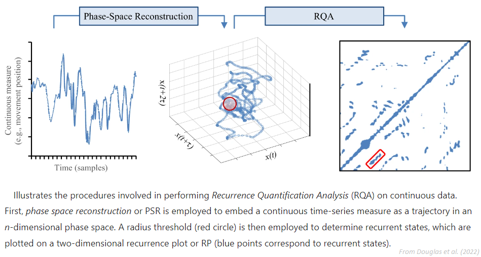
Illustration of RQA (Douglas et al., 2022).

Features include:

Recurrence rate (RR): Proportion of points that are labelled as recurrences. Depends on the radius r.
Determinism (DET): Proportion of recurrence points which form diagonal lines. Indicates autocorrelation.
Divergence (DIV): The inverse of the longest diagonal line length (LMax).
Laminarity (LAM): Proportion of recurrence points which form vertical lines. Indicates the amount of laminar phases (intermittency).
Trapping Time (TT): Average length of vertical black lines.
L: Average length of diagonal black lines. Average duration that a system is staying in the same state.
LEn: Entropy of diagonal lines lengths.
VMax: Longest vertical line length.
VEn: Entropy of vertical lines lengths.
W: Average white vertical line length.
WMax: Longest white vertical line length.
WEn: Entropy of white vertical lines lengths.
DeteRec: The ratio of determinism / recurrence rate.
LamiDet: The ratio of laminarity / determinism.
DiagRec: Diagonal Recurrence Rates, capturing the magnitude of autocorrelation at different lags, which is related to fractal fluctuations. See Tomashin et al. (2022), approach 3.

Note

More feature exist for RQA, such as the trend. We would like to add them, but we need help. Get in touch if you’re interested!

Parameters:

signal (Union[list, np.array, pd.Series]) – The signal (i.e., a time series) in the form of a vector of values.
delay (int) – Time delay (often denoted Tau $\tau$, sometimes referred to as lag) in samples. See complexity_delay() to estimate the optimal value for this parameter.
dimension (int) – Embedding Dimension (m, sometimes referred to as d or order). See complexity_dimension() to estimate the optimal value for this parameter.
tolerance (float) – Tolerance (often denoted as r), distance to consider two data points as similar. If "sd" (default), will be set to $0.2 * SD_{signal}$. See complexity_tolerance() to estimate the optimal value for this parameter.
min_linelength (int) – Minimum length of diagonal and vertical lines. Default to 2.
method (str) – Can be "pyrqa" to use the PyRQA package (requires to install it first).
show (bool) – Visualise recurrence matrix.

Returns:

rqa (DataFrame) – The RQA results.
info (dict) – A dictionary containing additional information regarding the parameters used to compute RQA.

Examples

In [1]: import neurokit2 as nk

In [2]: signal = nk.signal_simulate(duration=5, sampling_rate=100, frequency=[5, 6, 7], noise=0.2)

# RQA
In [3]: results, info = nk.complexity_rqa(signal, tolerance=1, show=True)

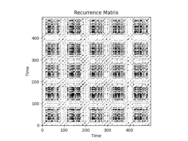
In [4]: results
Out[4]: 
   RecurrenceRate   DiagRec  Determinism  ...         W  WMax       WEn
0        0.236722 -0.028179      0.86042  ...  9.793781   300  2.961804

[1 rows x 14 columns]

# Compare to PyRQA
# results1, info = nk.complexity_rqa(signal, tolerance=1, show=True, method = "pyrqa")

References

Rawald, T., Sips, M., Marwan, N., & Dransch, D. (2014). Fast computation of recurrences in long time series. In Translational Recurrences (pp. 17-29). Springer, Cham.
Tomashin, A., Leonardi, G., & Wallot, S. (2022). Four Methods to Distinguish between Fractal Dimensions in Time Series through Recurrence Quantification Analysis. Entropy, 24(9), 1314.

Utilities#

fractal_mandelbrot()#

fractal_mandelbrot(size=1000, real_range=(-2, 2), imaginary_range=(-2, 2), threshold=4, iterations=25, buddha=False, show=False)[source]#

Mandelbrot (or a Buddhabrot) Fractal

Vectorized function to efficiently generate an array containing values corresponding to a Mandelbrot fractal.

Parameters:

size (int) – The size in pixels (corresponding to the width of the figure).
real_range (tuple) – The mandelbrot set is defined within the -2, 2 complex space (the real being the x-axis and the imaginary the y-axis). Adjusting these ranges can be used to pan, zoom and crop the figure.
imaginary_range (tuple) – The mandelbrot set is defined within the -2, 2 complex space (the real being the x-axis and the imaginary the y-axis). Adjusting these ranges can be used to pan, zoom and crop the figure.
iterations (int) – Number of iterations.
threshold (int) – The threshold used, increasing it will increase the sharpness (not used for buddhabrots).
buddha (bool) – Whether to return a buddhabrot.
show (bool) – Visualize the fractal.

Returns:

ndarray – Array of values.

Examples

Create the Mandelbrot fractal

In [1]: import neurokit2 as nk

In [2]: m = nk.fractal_mandelbrot(show=True)

$savefig/p_fractal_mandelbrot1.png$

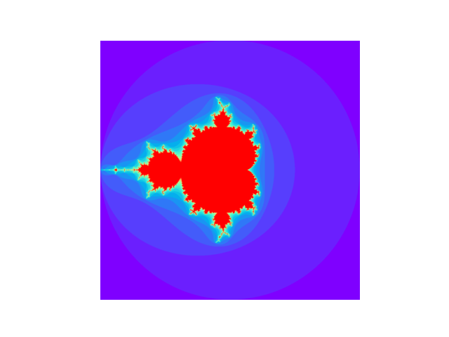
Zoom at the Seahorse Valley

In [3]: m = nk.fractal_mandelbrot(real_range=(-0.76, -0.74), imaginary_range=(0.09, 0.11),
   ...:                           iterations=100, show=True)
   ...: 

$savefig/p_fractal_mandelbrot2.png$

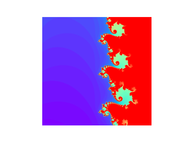
Draw manually

In [4]: import matplotlib.pyplot as plt

In [5]: m = nk.fractal_mandelbrot(real_range=(-2, 0.75), imaginary_range=(-1.25, 1.25))

In [6]: plt.imshow(m.T, cmap="viridis")
Out[6]: <matplotlib.image.AxesImage at 0x255c7e64700>

In [7]: plt.axis("off")
Out[7]: (-0.5, 908.5, 999.5, -0.5)

$savefig/p_fractal_mandelbrot3.png$

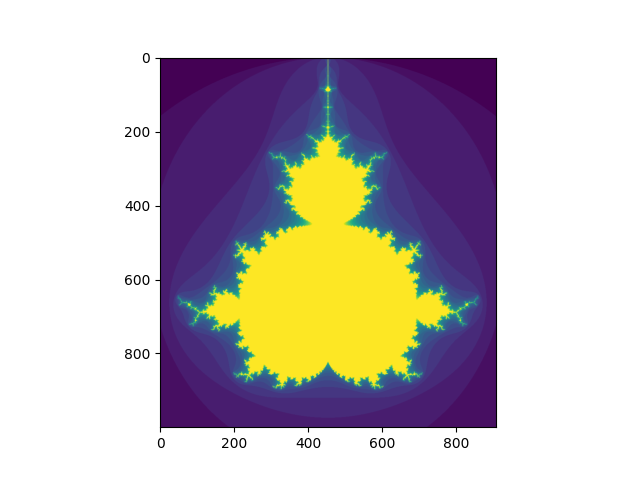
Generate a Buddhabrot fractal

In [8]: b = nk.fractal_mandelbrot(size=1500, real_range=(-2, 0.75), imaginary_range=(-1.25, 1.25),
   ...:                           buddha=True, iterations=200)
   ...: 

In [9]: plt.imshow(b.T, cmap="gray")
Out[9]: <matplotlib.image.AxesImage at 0x255c7e64b80>

In [10]: plt.axis("off")
Out[10]: (-0.5, 1363.5, 1499.5, -0.5)

$savefig/p_fractal_mandelbrot4.png$

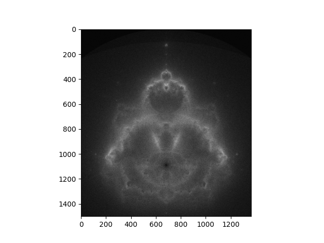
Mixed MandelBuddha

In [11]: m = nk.fractal_mandelbrot()

In [12]: b = nk.fractal_mandelbrot(buddha=True, iterations=200)

In [13]: mixed = m - b

In [14]: plt.imshow(mixed.T, cmap="gray")
Out[14]: <matplotlib.image.AxesImage at 0x255c3716920>

In [15]: plt.axis("off")
Out[15]: (-0.5, 999.5, 999.5, -0.5)

$savefig/p_fractal_mandelbrot5.png$

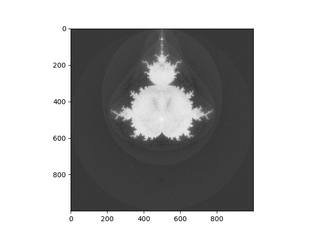
complexity_simulate()#

complexity_simulate(duration=10, sampling_rate=1000, method='ornstein', hurst_exponent=0.5, **kwargs)[source]#

Simulate chaotic time series

This function generates a chaotic signal using different algorithms and complex systems.

Mackey-Glass: Generates time series using the discrete approximation of the Mackey-Glass delay differential equation described by Grassberger & Procaccia (1983).
Ornstein-Uhlenbeck
Lorenz
Random walk

Parameters:

duration (int) – Desired length of duration (s).
sampling_rate (int) – The desired sampling rate (in Hz, i.e., samples/second).
duration (int) – The desired length in samples.
method (str) – The method. can be "hurst" for a (fractional) Ornstein-Uhlenbeck process, "lorenz" for the first dimension of a Lorenz system, "mackeyglass" to use the Mackey-Glass equation, or random to generate a random-walk.
hurst_exponent (float) – Defaults to 0.5.
**kwargs – Other arguments.

Returns:

array – Simulated complexity time series.

Examples

Lorenz System

In [1]: import neurokit2 as nk

In [2]: signal = nk.complexity_simulate(duration=5, sampling_rate=1000, method="lorenz")

In [3]: nk.signal_plot(signal)

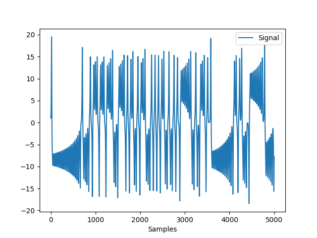
In [4]: nk.complexity_attractor(nk.complexity_embedding(signal, delay = 5), alpha=1, color="blue")
Out[4]: <Figure size 640x480 with 1 Axes>

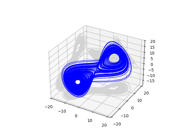
Ornstein System

In [5]: signal = nk.complexity_simulate(duration=30, sampling_rate=100, method="ornstein")

In [6]: nk.signal_plot(signal, color = "red")

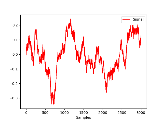
In [7]: nk.complexity_attractor(nk.complexity_embedding(signal, delay = 100), alpha=1, color="red")
Out[7]: <Figure size 640x480 with 1 Axes>

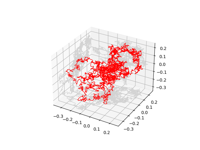
Mackey-Glass System

In [8]: signal = nk.complexity_simulate(duration=1, sampling_rate=1000, method="mackeyglass")

In [9]: nk.signal_plot(signal, color = "green")

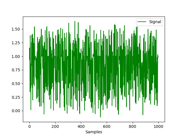
In [10]: nk.complexity_attractor(nk.complexity_embedding(signal, delay = 25), alpha=1, color="green")
Out[10]: <Figure size 640x480 with 1 Axes>

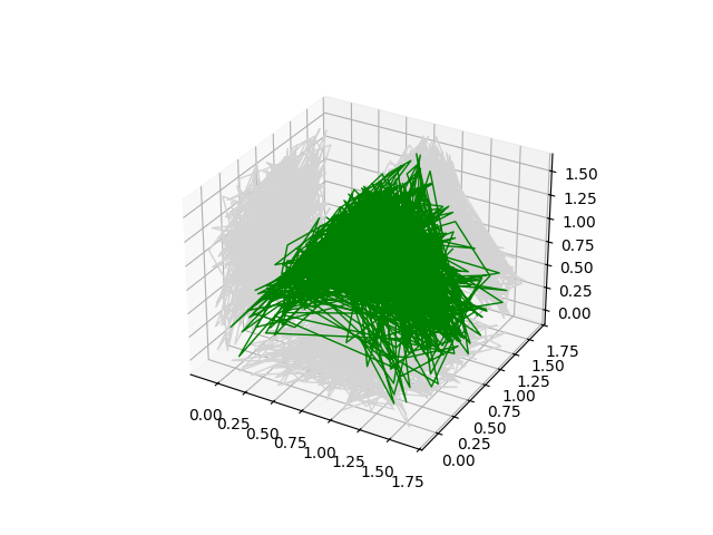
Random walk

In [11]: signal = nk.complexity_simulate(duration=30, sampling_rate=100, method="randomwalk")

In [12]: nk.signal_plot(signal, color = "orange")

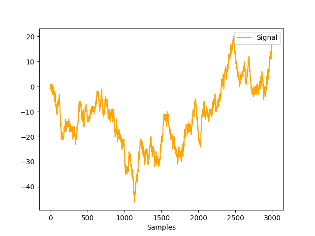
In [13]: nk.complexity_attractor(nk.complexity_embedding(signal, delay = 100), alpha=1, color="orange")
Out[13]: <Figure size 640x480 with 1 Axes>

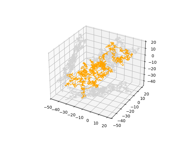
complexity_embedding()#

complexity_embedding(signal, delay=1, dimension=3, show=False, **kwargs)[source]#

Time-delay Embedding of a Signal

Time-delay embedding is one of the key concept of complexity science. It is based on the idea that a dynamical system can be described by a vector of numbers, called its ‘state’, that aims to provide a complete description of the system at some point in time. The set of all possible states is called the ‘state space’.

Takens’s (1981) embedding theorem suggests that a sequence of measurements of a dynamic system includes in itself all the information required to completely reconstruct the state space. Time-delay embedding attempts to identify the state s of the system at some time t by searching the past history of observations for similar states, and, by studying the evolution of similar states, infer information about the future of the system.

Attractors

How to visualize the dynamics of a system? A sequence of state values over time is called a trajectory. Depending on the system, different trajectories can evolve to a common subset of state space called an attractor. The presence and behavior of attractors gives intuition about the underlying dynamical system. We can visualize the system and its attractors by plotting the trajectory of many different initial state values and numerically integrating them to approximate their continuous time evolution on discrete computers.

Parameters:

signal (Union[list, np.array, pd.Series]) – The signal (i.e., a time series) in the form of a vector of values. Can also be a string, such as "lorenz" (Lorenz attractor), "rossler" (Rössler attractor), or "clifford" (Clifford attractor) to obtain a pre-defined attractor.
delay (int) – Time delay (often denoted Tau $\tau$, sometimes referred to as lag) in samples. See complexity_delay() to estimate the optimal value for this parameter.
dimension (int) – Embedding Dimension (m, sometimes referred to as d or order). See complexity_dimension() to estimate the optimal value for this parameter.
show (bool) – Plot the reconstructed attractor. See complexity_attractor() for details.
**kwargs – Other arguments to be passed to complexity_attractor().

Returns:

array – Embedded time-series, of shape length - (dimension - 1) * delay

Examples

Example 1: Understanding the output

The first columns contains the beginning of the signal, and the second column contains the values at t+2.

Example 2: 2D, 3D, and “4D” Attractors. Note that 3D attractors are slow to plot.

In the last 3D-attractor, the 4th dimension is represented by the color.

Example 3: Attractor of heart rate

ecg = nk.ecg_simulate(duration=60*4, sampling_rate=200) peaks, _ = nk.ecg_peaks(ecg, sampling_rate=200) signal = nk.ecg_rate(peaks, sampling_rate=200, desired_length=len(ecg))

@savefig p_complexity_embedding4.png scale=100% embedded = nk.complexity_embedding(signal, delay=250, dimension=2, show=True) @suppress plt.close()

References

Gautama, T., Mandic, D. P., & Van Hulle, M. M. (2003, April). A differential entropy based method for determining the optimal embedding parameters of a signal. In 2003 IEEE International Conference on Acoustics, Speech, and Signal Processing, 2003. Proceedings. (ICASSP’03). (Vol. 6, pp. VI-29). IEEE.
Takens, F. (1981). Detecting strange attractors in turbulence. In Dynamical systems and turbulence, Warwick 1980 (pp. 366-381). Springer, Berlin, Heidelberg.

complexity_attractor()#

complexity_attractor(embedded='lorenz', alpha='time', color='last_dim', shadows=True, linewidth=1, **kwargs)[source]#

Attractor Graph

Create an attractor graph from an embedded time series.

Parameters:

embedded (Union[str, np.ndarray]) – Output of complexity_embedding(). Can also be a string, such as "lorenz" (Lorenz attractor) or "rossler" (Rössler attractor).
alpha (Union[str, float]) – Transparency of the lines. If "time", the lines will be transparent as a function of time (slow).
color (str) – Color of the plot. If "last_dim", the last dimension (max 4th) of the embedded data will be used when the dimensions are higher than 2. Useful to visualize the depth (for 3-dimensions embedding), or the fourth dimension, but it is slow.
shadows (bool) – If True, 2D projections will be added to the sides of the 3D attractor.
linewidth (float) – Set the line width in points.
**kwargs – Additional keyword arguments are passed to the color palette (e.g., name="plasma"), or to the Lorenz system simulator, such as duration (default = 100), sampling_rate (default = 10), sigma (default = 10), beta (default = 8/3), rho (default = 28).

See also

complexity_embeddding

Examples

Lorenz attractors

In [1]: import neurokit2 as nk

In [2]: fig = nk.complexity_attractor(color = "last_dim", alpha="time", duration=1)

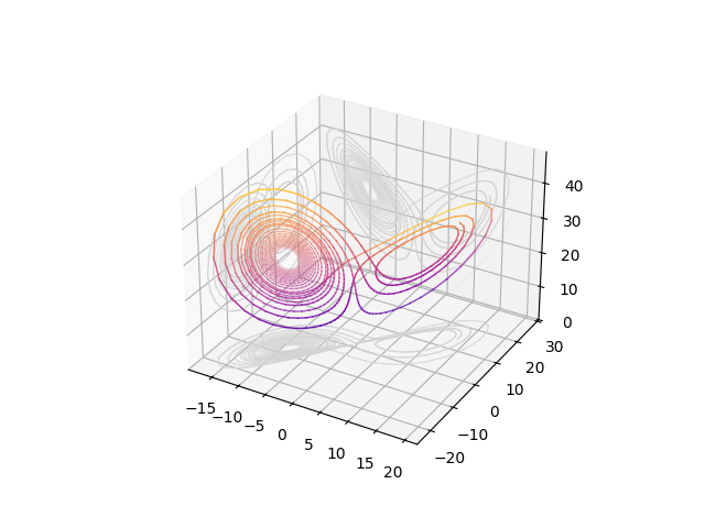
# Fast result (fixed alpha and color)
In [3]: fig = nk.complexity_attractor(color = "red", alpha=1, sampling_rate=5000, linewidth=0.2)

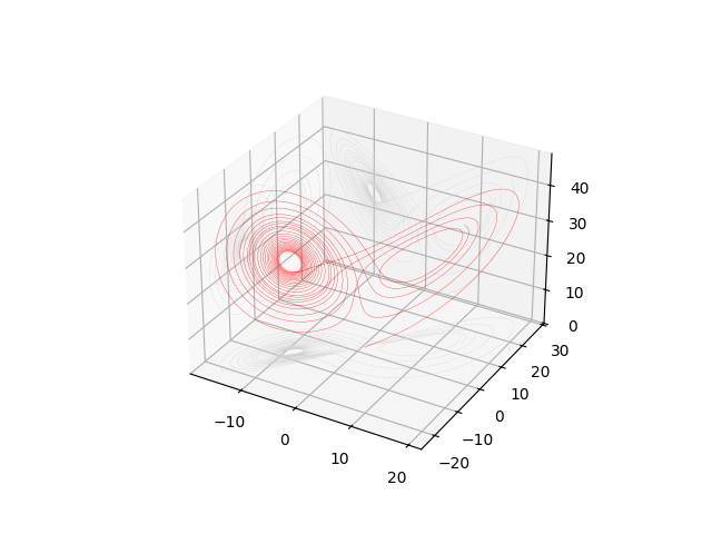
Rössler attractors

In [4]: nk.complexity_attractor("rossler", color = "blue", alpha=1, sampling_rate=5000)
Out[4]: <Figure size 640x480 with 1 Axes>

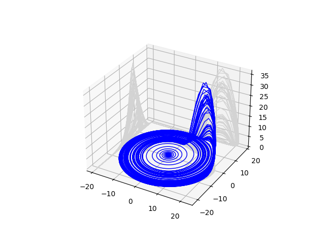
2D Attractors using a signal

# Simulate Signal
In [5]: signal = nk.signal_simulate(duration=10, sampling_rate=100, frequency = [0.1, 5, 7, 10])

# 2D Attractor
In [6]: embedded = nk.complexity_embedding(signal, delay = 3, dimension = 2)

# Fast (fixed alpha and color)
In [7]: nk.complexity_attractor(embedded, color = "red", alpha = 1)
Out[7]: <Figure size 640x480 with 1 Axes>

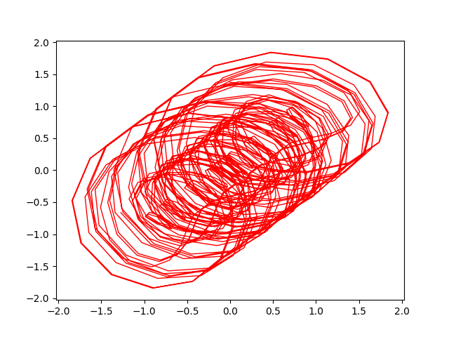
# Slow
In [8]: nk.complexity_attractor(embedded, color = "last_dim", alpha = "time")
Out[8]: <Figure size 640x480 with 1 Axes>

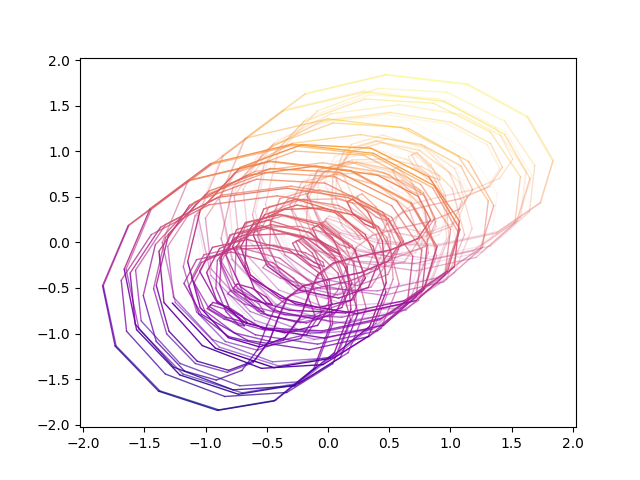
3D Attractors using a signal

# 3D Attractor
In [9]: embedded = nk.complexity_embedding(signal, delay = 3, dimension = 3)

# Fast (fixed alpha and color)
In [10]: nk.complexity_attractor(embedded, color = "red", alpha = 1)
Out[10]: <Figure size 640x480 with 1 Axes>

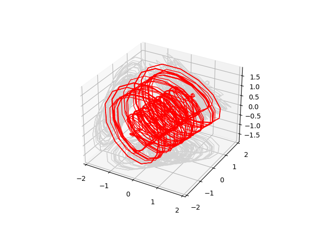
# Slow
In [11]: nk.complexity_attractor(embedded, color = "last_dim", alpha = "time")
Out[11]: <Figure size 640x480 with 1 Axes>

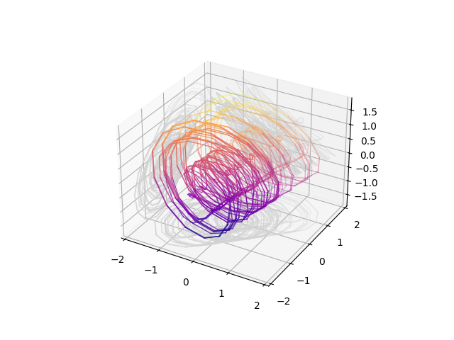
Animated Rotation

In [12]: import matplotlib.animation as animation

In [13]: import IPython

In [14]: fig = nk.complexity_attractor(embedded, color = "black", alpha = 0.5, shadows=False)

In [15]: ax = fig.get_axes()[0]

In [16]: def rotate(angle):
   ....:     ax.view_init(azim=angle)
   ....: anim = animation.FuncAnimation(fig, rotate, frames=np.arange(0, 361, 10), interval=10)
   ....: IPython.display.HTML(anim.to_jshtml())
   ....: 
Out[16]: <IPython.core.display.HTML object>

complexity_symbolize#

complexity_symbolize(signal, method='mean', c=3, random_state=None, show=False, **kwargs)[source]#

Signal Symbolization and Discretization

Many complexity indices are made to assess the recurrence and predictability of discrete - symbolic - states. As such, continuous signals must be transformed into such discrete sequence.

For instance, one of the easiest way is to split the signal values into two categories, above and below the mean, resulting in a sequence of A and B. More complex methods have been developped to that end.

Method ‘A’ binarizes the signal by higher vs. lower values as compated to the signal’s mean. Equivalent tp method="mean" (method="median" is also valid).
Method ‘B’ uses values that are within the mean +/- 1 SD band vs. values that are outside this band.
Method ‘C’ computes the difference between consecutive samples and binarizes depending on their sign.
Method ‘D’ forms separates consecutive samples that exceed 1 signal’s SD from the others smaller changes.
Method ‘r’ is based on the concept of *tolerance*, and will separate consecutive samples that exceed a given tolerance threshold, by default $0.2 * SD$. See complexity_tolerance() for more details.
Binning: If an integer n is passed, will bin the signal into n equal-width bins. Requires to specify c.
MEP: Maximum Entropy Partitioning. Requires to specify c.
NCDF: Please help us to improve the documentation here. Requires to specify c.
Linear: Please help us to improve the documentation here. Requires to specify c.
Uniform: Please help us to improve the documentation here. Requires to specify c.
kmeans: k-means clustering. Requires to specify c.

Parameters:

signal (Union[list, np.array, pd.Series]) – The signal (i.e., a time series) in the form of a vector of values.
method (str or int) – Method of symbolization. Can be one of "A" (default), "B", "C", "D", "r", "Binning", "MEP", "NCDF", "linear", "uniform", "kmeans", "equal", or None to skip the process (for instance, in cases when the binarization has already been done before).

See complexity_symbolize() for details.
c (int) – Number of symbols c, used in some algorithms.
random_state (None, int, numpy.random.RandomState or numpy.random.Generator) – Seed for the random number generator. See misc.check_random_state() for further information.
show (bool) – Plot the reconstructed attractor. See complexity_attractor() for details.
**kwargs – Other arguments to be passed to complexity_attractor().

Returns:

array – A symbolic sequence made of discrete states (e.g., 0 and 1).

See also

entropy_shannon, entropy_cumulative_residual, fractal_petrosian

Examples

In [1]: import neurokit2 as nk

In [2]: signal = nk.signal_simulate(duration=2, frequency=[5, 12])

# Method "A" is equivalent to "mean"
In [3]: symbolic = nk.complexity_symbolize(signal, method = "A", show=True)

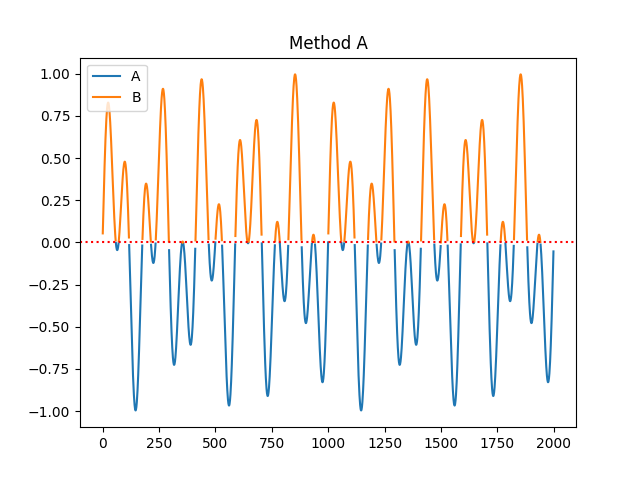
In [4]: symbolic = nk.complexity_symbolize(signal, method = "B", show=True)

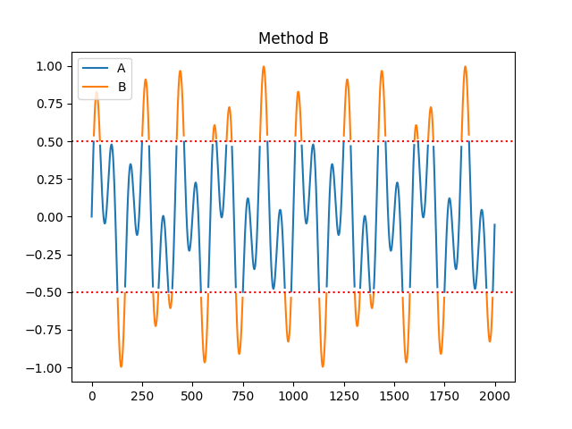
In [5]: symbolic = nk.complexity_symbolize(signal, method = "C", show=True)

In [6]: signal = nk.signal_simulate(duration=2, frequency=[5], noise = 0.1)

In [7]: symbolic = nk.complexity_symbolize(signal, method = "D", show=True)

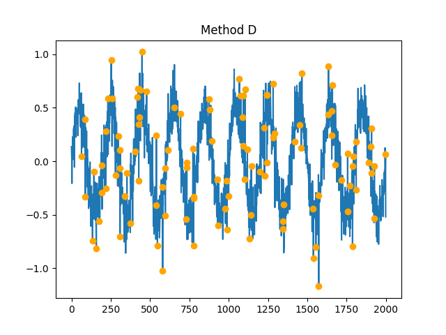
In [8]: symbolic = nk.complexity_symbolize(signal, method = "r", show=True)

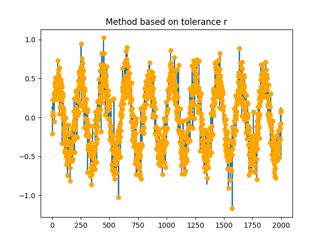
In [9]: symbolic = nk.complexity_symbolize(signal, method = "binning", c=3, show=True)

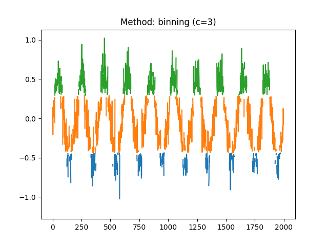
In [10]: symbolic = nk.complexity_symbolize(signal, method = "MEP", c=3, show=True)

In [11]: symbolic = nk.complexity_symbolize(signal, method = "NCDF", c=3, show=True)

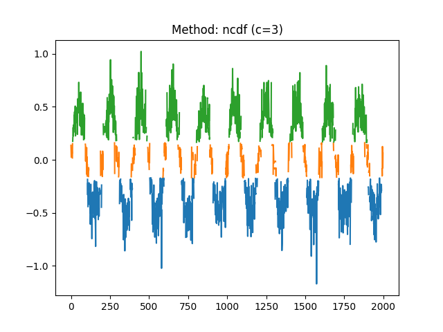
In [12]: symbolic = nk.complexity_symbolize(signal, method = "linear", c=5, show=True)

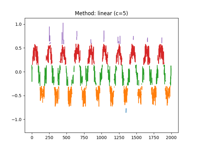
In [13]: symbolic = nk.complexity_symbolize(signal, method = "equal", c=5, show=True)

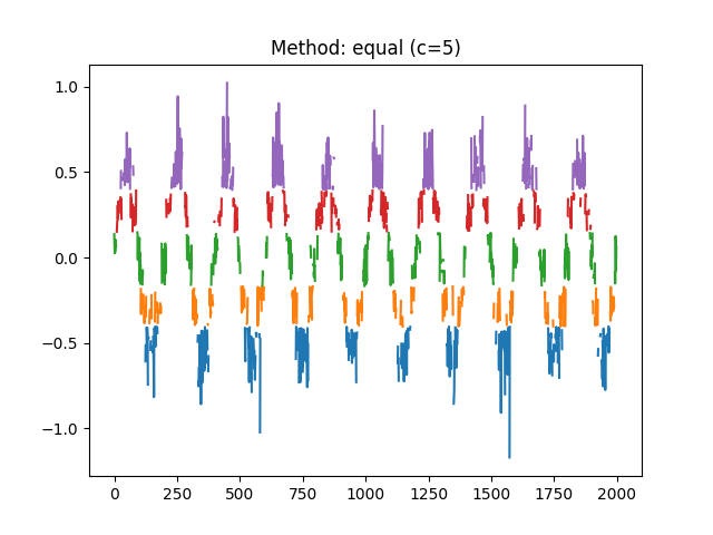
In [14]: symbolic = nk.complexity_symbolize(signal, method = "kmeans", c=5, random_state=42, show=True)

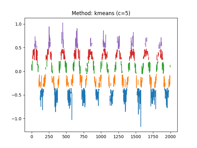
complexity_coarsegraining()#

complexity_coarsegraining(signal, scale=2, method='nonoverlapping', show=False, **kwargs)[source]#

Coarse-graining of a signal

The goal of coarse-graining is to represent the signal at a different “scale”. The coarse-grained time series for a scale factor Tau ($\tau$) are obtained by averaging non-overlapping windows of size Tau. In most of the complexity metrics, multiple coarse-grained segments are constructed for a given signal, to represent the signal at different scales (hence the “multiscale” adjective).

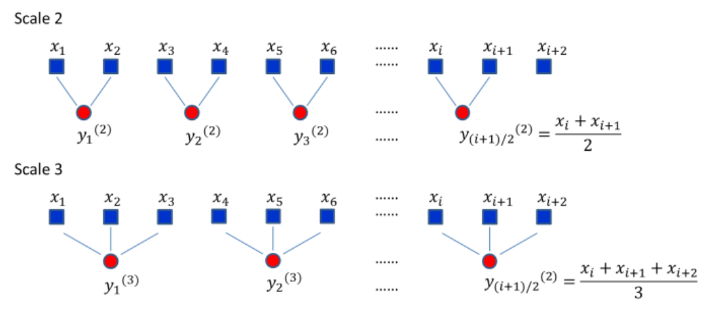
This coarse-graining procedure is similar to moving averaging and the decimation of the original time series. The length of each coarse-grained time series is N/Tau. For scale = 1, the coarse-grained time series is simply the original time series itself.

The coarse graining procedure (used for instance in MSE) is considered a shortcoming that decreases the entropy rate artificially (Nikulin, 2004). One of the core issue is that the length of coarse-grained signals becomes smaller as the scale increases.

To address this issue of length, several methods have been proposed, such as adaptive resampling (Liu et al. 2012), moving average (Wu et al. 2013), or timeshift (Wu et al. 2013).

Non-overlapping (default): The coarse-grained time series are constructed by averaging non-overlapping windows of given size.
Interpolate: Interpolates (i.e., resamples) the coarse-grained time series to match the original signal length (currently using a monotonic cubic method, but let us know if you have any opinion on that).
Moving average: The coarse-grained time series via a moving average.
Time-shift: For each scale, a k number of coarse-grained vectors are constructed (see Figure below). Somewhat similar to moving-average, with the difference that the time lag creates new vectors.

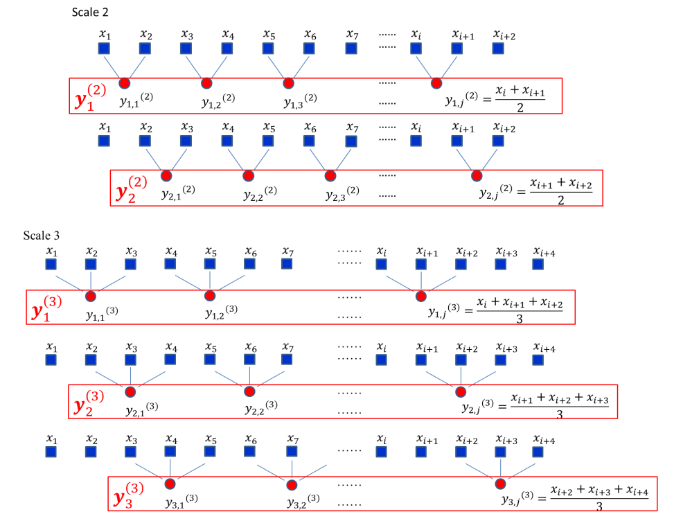
Parameters:

signal (Union[list, np.array, pd.Series]) – The signal (i.e., a time series) in the form of a vector of values.
scale (int) – The size of the windows that the signal is divided into. Also referred to as Tau $\tau$, it represents the scale factor and corresponds to the amount of coarsegraining.
method (str) – Can be "nonoverlapping", "rolling", "interpolate", or "timeshift".
show (bool) – If True, will show the coarse-grained signal.
**kwargs – Other arguments (not used currently).

Returns:

array – The coarse-grained signal.

Examples

Simple examples .. ipython:: python

import neurokit2 as nk

signal = [0, 2, 4, 6, 8, 10] nk.complexity_coarsegraining(signal, scale=2)

signal = [0, 1, 2, 0, 1] nk.complexity_coarsegraining(signal, scale=3)

nk.complexity_coarsegraining(signal=range(10), method=”interpolate”) nk.complexity_coarsegraining(signal=range(10), method=”rolling”)

Simulated signal .. ipython:: python

signal = nk.signal_simulate(duration=2, frequency=[5, 20])

@savefig p_complexity_coarsegraining1.png scale=100% coarsegrained = nk.complexity_coarsegraining(signal, scale=40, show=True) @suppress plt.close()

In [1]: coarsegrained = nk.complexity_coarsegraining(signal, scale=40, method="interpolate", show=True)

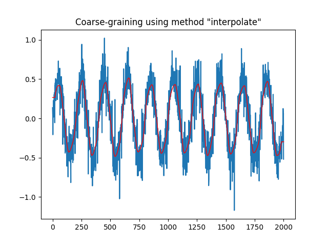
savefig/p_complexity_coarsegraining2.png

In [2]: coarsegrained = nk.complexity_coarsegraining(signal, scale=40, method="rolling", show=True)

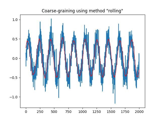
savefig/p_complexity_coarsegraining3.png

In [3]: signal = nk.signal_simulate(duration=0.5, frequency=[5, 20])

In [4]: coarsegrained = nk.complexity_coarsegraining(signal, scale=30, method="timeshift", show=True)

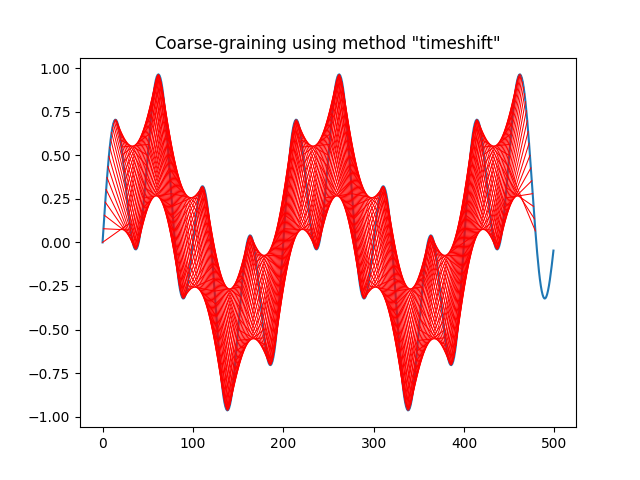
savefig/p_complexity_coarsegraining4.png

Benchmarking .. ipython:: python

signal = nk.signal_simulate(duration=10, frequency=5) scale = 2 x_pd = pd.Series(signal).rolling(window=scale).mean().values[scale-1::scale] x_nk = nk.complexity_coarsegraining(signal, scale=scale) np.allclose(x_pd - x_nk, 0)

%timeit x_pd = pd.Series(signal).rolling(window=scale).mean().values[scale-1::scale] %timeit x_nk = nk.complexity_coarsegraining(signal, scale=scale)

signal = nk.signal_simulate(duration=30, frequency=5) scale = 3

x_pd = pd.Series(signal).rolling(window=scale).mean().values[scale-1::] x_nk = nk.complexity_coarsegraining(signal, scale=scale, rolling=True) np.allclose(x_pd - x_nk[1:-1], 0)

%timeit pd.Series(signal).rolling(window=scale).mean().values[scale-1::] %timeit nk.complexity_coarsegraining(signal, scale=scale, rolling=True)

References

Su, C., Liang, Z., Li, X., Li, D., Li, Y., & Ursino, M. (2016). A comparison of multiscale permutation entropy measures in on-line depth of anesthesia monitoring. PLoS One, 11(10), e0164104.
Nikulin, V. V., & Brismar, T. (2004). Comment on “Multiscale entropy analysis of complex physiologic time series”” Physical review letters, 92(8), 089803.
Liu, Q., Wei, Q., Fan, S. Z., Lu, C. W., Lin, T. Y., Abbod, M. F., & Shieh, J. S. (2012). Adaptive computation of multiscale entropy and its application in EEG signals for monitoring depth of anesthesia during surgery. Entropy, 14(6), 978-992.
Wu, S. D., Wu, C. W., Lee, K. Y., & Lin, S. G. (2013). Modified multiscale entropy for short-term time series analysis. Physica A: Statistical Mechanics and its Applications, 392 (23), 5865-5873.
Wu, S. D., Wu, C. W., Lin, S. G., Wang, C. C., & Lee, K. Y. (2013). Time series analysis using composite multiscale entropy. Entropy, 15(3), 1069-1084.

complexity_ordinalpatterns()#

complexity_ordinalpatterns(signal, delay=1, dimension=3, algorithm='quicksort', **kwargs)[source]#

Find Ordinal Patterns for Permutation Procedures

The seminal work by Bandt and Pompe (2002) introduced a symbolization approach to obtain a sequence of ordinal patterns (permutations) from continuous data. It is used in permutation entropy and its different variants.

Parameters:

signal (Union[list, np.array, pd.Series]) – The signal (i.e., a time series) in the form of a vector of values.
delay (int) – Time delay (often denoted Tau $\tau$, sometimes referred to as lag) in samples. See complexity_delay() to estimate the optimal value for this parameter.
dimension (int) – Embedding Dimension (m, sometimes referred to as d or order). See complexity_dimension() to estimate the optimal value for this parameter.
algorithm (str) – Can be "quicksort" (default) or "bubblesort" (used in Bubble Entropy).

Returns:

array – Ordinal patterns.
vector – Frequencies of each ordinal pattern.
dict – A dictionary containing additional elements.

Examples

Example given by Bandt and Pompe (2002):

In [1]: import neurokit2 as nk

In [2]: signal = [4, 7, 9, 10, 6, 11, 3]

In [3]: patterns, info = nk.complexity_ordinalpatterns(signal, delay=1, dimension=3)

In [4]: patterns
Out[4]: 
array([[0, 1, 2],
       [1, 0, 2],
       [2, 0, 1]], dtype=int64)

In [5]: info["Frequencies"]
Out[5]: array([0.4, 0.2, 0.4])

In [6]: signal = [4, 7, 9, 10, 6, 5, 3, 6, 8, 9, 5, 1, 0]

In [7]: patterns, info = nk.complexity_ordinalpatterns(signal, algorithm="bubblesort")

In [8]: info["Frequencies"]
Out[8]: array([0.36363636, 0.09090909, 0.18181818, 0.36363636])

References

Bandt, C., & Pompe, B. (2002). Permutation entropy: a natural complexity measure for time series. Physical review letters, 88(17), 174102.
Manis, G., Aktaruzzaman, M. D., & Sassi, R. (2017). Bubble entropy: An entropy almost free of parameters. IEEE Transactions on Biomedical Engineering, 64(11), 2711-2718.

recurrence_matrix()#

recurrence_matrix(signal, delay=1, dimension=3, tolerance='default', show=False)[source]#

Recurrence Matrix

Fast Python implementation of recurrence matrix (tested against pyRQA). Returns a tuple with the recurrence matrix (made of 0s and 1s) and the distance matrix (the non-binarized version of the former).

It is used in Recurrence Quantification Analysis (RQA).

Parameters:

signal (Union[list, np.ndarray, pd.Series]) – The signal (i.e., a time series) in the form of a vector of values.
delay (int) – Time delay (often denoted Tau $\tau$, sometimes referred to as lag) in samples. See complexity_delay() to estimate the optimal value for this parameter.
dimension (int) – Embedding Dimension (m, sometimes referred to as d or order). See complexity_dimension() to estimate the optimal value for this parameter.
tolerance (float) – Tolerance (often denoted as r), distance to consider two data points as similar. If "sd" (default), will be set to $0.2 * SD_{signal}$. See complexity_tolerance() to estimate the optimal value for this parameter. A rule of thumb is to set r so that the percentage of points classified as recurrences is about 2-5%.
show (bool) – Visualise recurrence matrix.

Returns:

np.ndarray – The recurrence matrix.
np.ndarray – The distance matrix.

Examples

In [1]: import neurokit2 as nk

In [2]: signal = nk.signal_simulate(duration=2, sampling_rate=100, frequency=[5, 6], noise=0.01)

# Default r
In [3]: rc, _ = nk.recurrence_matrix(signal, show=True)

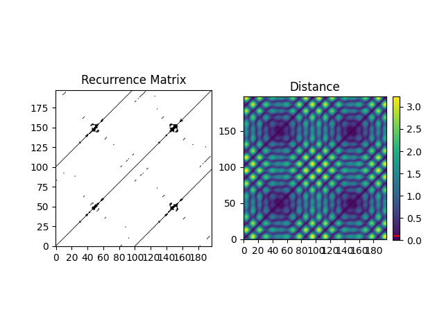
# Larger radius
In [4]: rc, d = nk.recurrence_matrix(signal, tolerance=0.5, show=True)

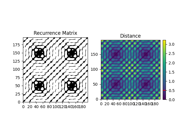
# Optimization of tolerance via recurrence matrix
In [5]: tol, _ = nk.complexity_tolerance(signal, dimension=1, delay=3, method="recurrence", show=True)

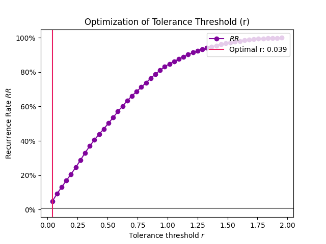
In [6]: rc, d = nk.recurrence_matrix(signal, tolerance=tol, show=True)

References

Rawald, T., Sips, M., Marwan, N., & Dransch, D. (2014). Fast computation of recurrences in long time series. In Translational Recurrences (pp. 17-29). Springer, Cham.
Dabiré, H., Mestivier, D., Jarnet, J., Safar, M. E., & Chau, N. P. (1998). Quantification of sympathetic and parasympathetic tones by nonlinear indexes in normotensive rats. American Journal of Physiology-Heart and Circulatory Physiology, 275(4), H1290-H1297.

Joint/Multivariate#

entropy_shannon_joint()#

entropy_shannon_joint(x, y, base=2)[source]#

Shannon’s Joint Entropy

The joint entropy measures how much entropy is contained in a joint system of two random variables.

Parameters:

x (Union[list, np.array, pd.Series]) – A symbolic sequence in the form of a vector of values.
y (Union[list, np.array, pd.Series]) – Another symbolic sequence with the same values.
base (float) – The logarithmic base to use, defaults to 2. Note that scipy.stats.entropy() uses np.e as default (the natural logarithm).

Returns:

float – The Shannon joint entropy.
dict – A dictionary containing additional information regarding the parameters used to compute Shannon entropy.

See also

entropy_shannon

Examples

In [1]: import neurokit2 as nk

In [2]: x = ["A", "A", "A", "B", "A", "B"]

In [3]: y = ["A", "B", "A", "A", "A", "A"]

In [4]: jen, _ = nk.entropy_shannon_joint(x, y)

In [5]: jen
Out[5]: 0.118714603408425

Complexity, Fractals, and Entropy

Contents

Complexity, Fractals, and Entropy#

Main#

complexity()#

Parameters Choice#

complexity_delay()#

complexity_dimension()#

complexity_tolerance()#

complexity_k()#

Fractal Dimension#

fractal_katz()#

fractal_linelength()#

fractal_petrosian()#

fractal_sevcik()#

fractal_nld()#

fractal_psdslope()#

fractal_higuchi()#

fractal_density()#

fractal_hurst()#

fractal_correlation()#

fractal_dfa()#

fractal_tmf()#

Entropy#

entropy_shannon()#

entropy_maximum()#

entropy_differential()#

entropy_power()#

entropy_tsallis()#

entropy_renyi()#

entropy_approximate()#

entropy_sample()#

entropy_quadratic()#

entropy_cumulativeresidual()#

entropy_rate()#

entropy_svd()#

entropy_kl()#

entropy_spectral()#

entropy_phase()#

entropy_grid()#

entropy_attention()#

entropy_increment()#

entropy_slope()#

entropy_symbolicdynamic()#

entropy_dispersion()#

entropy_ofentropy()#

entropy_permutation()#

entropy_bubble()#

entropy_range()#

entropy_fuzzy()#

entropy_multiscale()#

entropy_hierarchical()#

Other indices#

fisher_information()#

fishershannon_information()#

mutual_information()#

complexity_hjorth()#

complexity_decorrelation()#

complexity_lempelziv()#

complexity_relativeroughness()#

complexity_lyapunov()#

complexity_rqa()#

Utilities#

fractal_mandelbrot()#

complexity_simulate()#

complexity_embedding()#

complexity_attractor()#

complexity_symbolize#

complexity_coarsegraining()#

complexity_ordinalpatterns()#

recurrence_matrix()#

Joint/Multivariate#

entropy_shannon_joint()#