
Stats#
Utilities#
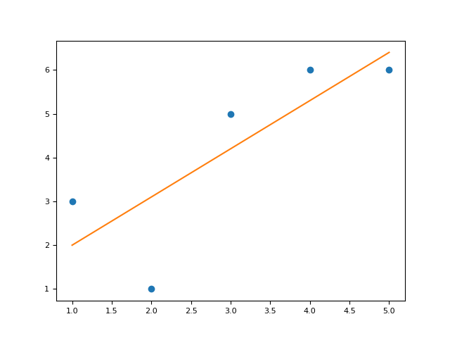
correlation()#
- cor(x, y, method='pearson', show=False)[source]#
Density estimation
Computes kernel density estimates.
- Parameters:
x (Union[list, np.array, pd.Series]) – Vectors of values.
y (Union[list, np.array, pd.Series]) – Vectors of values.
method (str) – Correlation method. Can be one of
"pearson","spearman","kendall".show (bool) – Draw a scatterplot with a regression line.
- Returns:
r – The correlation coefficient.
Examples
In [1]: import neurokit2 as nk

In [2]: x = [1, 2, 3, 4, 5]

In [3]: y = [3, 1, 5, 6, 6]

In [4]: corr = nk.cor(x, y, method="pearson", show=True)

In [5]: corr
Out[5]: np.float64(0.8022574532384201)
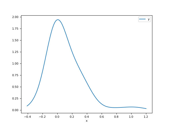
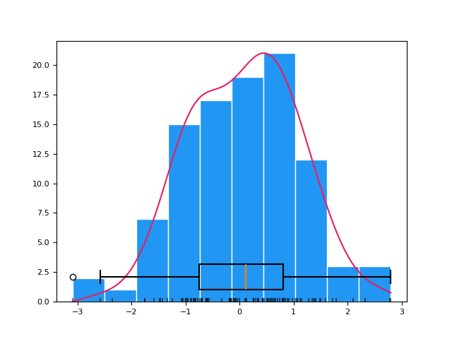
density()#
- density(x, desired_length=100, bandwidth='Scott', show=False, **kwargs)[source]#
Density estimation.
Computes kernel density estimates.
- Parameters:
x (Union[list, np.array, pd.Series]) – A vector of values.
desired_length (int) – The amount of values in the returned density estimation.
bandwidth (float) – Passed to the
methodargument from thedensity_bandwidth()function.show (bool) – Display the density plot.
**kwargs – Additional arguments to be passed to
density_bandwidth().
- Returns:
x – The x axis of the density estimation.
y – The y axis of the density estimation.
See also
density_bandwidthExamples
In [1]: import neurokit2 as nk

In [2]: signal = nk.ecg_simulate(duration=20)

In [3]: x, y = nk.density(signal, bandwidth=0.5, show=True)
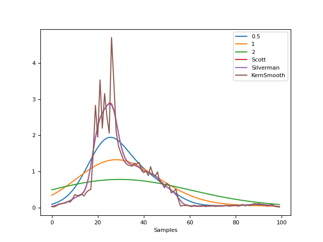
# Bandwidth comparison
In [4]: _, y2 = nk.density(signal, bandwidth=1)

In [5]: _, y3 = nk.density(signal, bandwidth=2)

In [6]: _, y4 = nk.density(signal, bandwidth="scott")

In [7]: _, y5 = nk.density(signal, bandwidth="silverman")

In [8]: _, y6 = nk.density(signal, bandwidth="kernsmooth")

In [9]: nk.signal_plot([y, y2, y3, y4, y5, y6],
   ...:                labels=["0.5", "1", "2", "Scott", "Silverman", "KernSmooth"])
   ...:
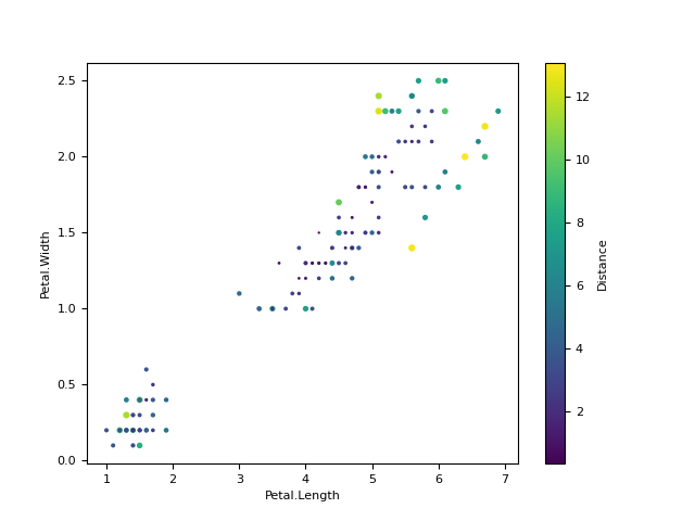
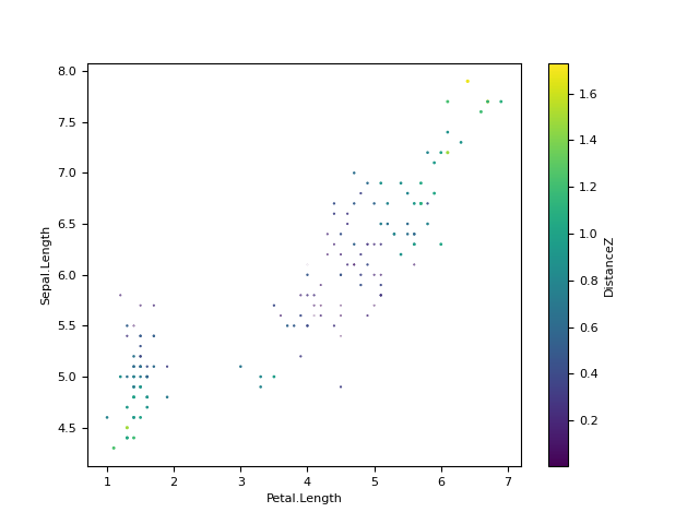
distance()#
- distance(X=None, method='mahalanobis')[source]#
Distance
Compute distance using different metrics.
- Parameters:
X (array or DataFrame) – A dataframe of values.
method (str) – The method to use. One of
"mahalanobis"or"mean"for the average distance from the mean.
- Returns:
array – Vector containing the distance values.
Examples
In [1]: import neurokit2 as nk

# Load the iris dataset
In [2]: data = nk.data("iris").drop("Species", axis=1)

In [3]: data["Distance"] = nk.distance(data, method="mahalanobis")

In [4]: fig = data.plot(x="Petal.Length", y="Petal.Width", s="Distance", c="Distance", kind="scatter")
In [5]: data["DistanceZ"] = np.abs(nk.distance(data.drop("Distance", axis=1), method="mean"))

In [6]: fig = data.plot(x="Petal.Length", y="Sepal.Length", s="DistanceZ", c="DistanceZ", kind="scatter")
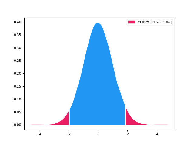
hdi()#
- hdi(x, ci=0.95, show=False, **kwargs)[source]#
Highest Density Interval (HDI)
Compute the Highest Density Interval (HDI) of a distribution. All points within this interval have a higher probability density than points outside the interval. The HDI can be used in the context of uncertainty characterisation of posterior distributions (in the Bayesian farmework) as Credible Interval (CI). Unlike equal-tailed intervals that typically exclude 2.5% from each tail of the distribution and always include the median, the HDI is not equal-tailed and therefore always includes the mode(s) of posterior distributions.
- Parameters:
x (Union[list, np.array, pd.Series]) – A vector of values.
ci (float) – Value of probability of the (credible) interval - CI (between 0 and 1) to be estimated. Default to .95 (95%).
show (bool) – If
True, the function will produce a figure.**kwargs (Line2D properties) – Other arguments to be passed to
nk.density().
See also
- Returns:
float(s) – The HDI low and high limits.
fig – Distribution plot.
Examples
In [1]: import numpy as np

In [2]: import neurokit2 as nk

In [3]: x = np.random.normal(loc=0, scale=1, size=100000)

In [4]: ci_min, ci_high = nk.hdi(x, ci=0.95, show=True)
mad()#
- mad(x, constant=1.4826, **kwargs)[source]#
Median Absolute Deviation: a “robust” version of standard deviation
- Parameters:
x (Union[list, np.array, pd.Series]) – A vector of values.
constant (float) – Scale factor. Use 1.4826 for results similar to default R.
- Returns:
float – The MAD.
Examples
In [1]: import neurokit2 as nk

In [2]: nk.mad([2, 8, 7, 5, 4, 12, 5, 1])
Out[2]: np.float64(3.7064999999999997)
References
rescale()#
- rescale(data, to=[0, 1], scale=None)[source]#
Rescale data
Rescale a numeric variable to a new range.
- Parameters:
data (Union[list, np.array, pd.Series]) – Raw data.
to (list) – New range of values of the data after rescaling. Must be a list or tuple of two values. If more values, the function will assume it is another signal and will derive the min and max from it.
scale (list) – A list or tuple of two values specifying the actual range of the data. If
None, the minimum and the maximum of the provided data will be used.
- Returns:
list – The rescaled values.
Examples
In [1]: import neurokit2 as nk

# Normalize to 0-1
In [2]: nk.rescale([3, 1, 2, 4, 6], to=[0, 1])
Out[2]:
[np.float64(0.4),
 np.float64(0.0),
 np.float64(0.2),
 np.float64(0.6000000000000001),
 np.float64(1.0)]

# Rescale to 0-1, but specify that 0 corresponds to another value that the
# minimum of the data.
In [3]: nk.rescale([3, 1, 2, 4, 6], to=[0, 1], scale=[0, 6])
Out[3]:
[np.float64(0.5),
 np.float64(0.16666666666666666),
 np.float64(0.3333333333333333),
 np.float64(0.6666666666666666),
 np.float64(1.0)]

# Rescale to 0-4 (the min-max of another signal)
In [4]: nk.rescale([3, 1, 2, 4, 6], to=[0, 1, 3, 4])
Out[4]:
[np.float64(1.6),
 np.float64(0.0),
 np.float64(0.8),
 np.float64(2.4000000000000004),
 np.float64(4.0)]
standardize()#
- standardize(data, robust=False, window=None, **kwargs)[source]#
Standardization of data
Performs a standardization of data (Z-scoring), i.e., centering and scaling, so that the data is expressed in terms of standard deviation (i.e., mean = 0, SD = 1) or Median Absolute Deviance (median = 0, MAD = 1).
- Parameters:
data (Union[list, np.array, pd.Series]) – Raw data.
robust (bool) – If
True, centering is done by substracting the median from the variables and dividing it by the median absolute deviation (MAD). IfFalse, variables are standardized by substracting the mean and dividing it by the standard deviation (SD).window (int) – Perform a rolling window standardization, i.e., apply a standardization on a window of the specified number of samples that rolls along the main axis of the signal. Can be used for complex detrending.
**kwargs (optional) – Other arguments to be passed to
pandas.rolling().
- Returns:
list – The standardized values.
Examples
In [1]: import neurokit2 as nk

In [2]: import pandas as pd

# Simple example
In [3]: nk.standardize([3, 1, 2, 4, 6, np.nan])
Out[3]:
[np.float64(-0.10397504898200735),
 np.float64(-1.14372553880208),
 np.float64(-0.6238502938920437),
 np.float64(0.41590019592802896),
 np.float64(1.4556506857481015),
 np.float64(nan)]

In [4]: nk.standardize([3, 1, 2, 4, 6, np.nan], robust=True)
Out[4]:
[np.float64(0.0),
 np.float64(-1.3489815189531904),
 np.float64(-0.6744907594765952),
 np.float64(0.6744907594765952),
 np.float64(2.023472278429786),
 np.float64(nan)]

In [5]: nk.standardize(np.array([[1, 2, 3, 4], [5, 6, 7, 8]]).T)
Out[5]:
array([[-1.161895  , -1.161895  ],
       [-0.38729833, -0.38729833],
       [ 0.38729833,  0.38729833],
       [ 1.161895  ,  1.161895  ]])

In [6]: nk.standardize(pd.DataFrame({"A": [3, 1, 2, 4, 6, np.nan],
   ...:                              "B": [3, 1, 2, 4, 6, 5]}))
   ...:
Out[6]:
          A         B
0 -0.103975 -0.267261
1 -1.143726 -1.336306
2 -0.623850 -0.801784
3  0.415900  0.267261
4  1.455651  1.336306
5       NaN  0.801784

# Rolling standardization of a signal
In [7]: signal = nk.signal_simulate(frequency=[0.1, 2], sampling_rate=200)

In [8]: z = nk.standardize(signal, window=200)

In [9]: nk.signal_plot([signal, z], standardize=True)
summary()#
Clustering#
cluster()#
- cluster(data, method='kmeans', n_clusters=2, random_state=None, optimize=False, **kwargs)[source]#
Data Clustering
Performs clustering of data using different algorithms.
kmod: Modified k-means algorithm.
kmeans: Normal k-means.
kmedoids: k-medoids clustering, a more stable version of k-means.
pca: Principal Component Analysis.
ica: Independent Component Analysis.
aahc: Atomize and Agglomerate Hierarchical Clustering. Computationally heavy.
hierarchical
spectral
mixture
mixturebayesian
See
sklearnfor methods details.- Parameters:
data (np.ndarray) – Matrix array of data (E.g., an array (channels, times) of M/EEG data).
method (str) – The algorithm for clustering. Can be one of
"kmeans"(default),"kmod","kmedoids","pca","ica","aahc","hierarchical","spectral","mixture","mixturebayesian".n_clusters (int) – The desired number of clusters.
random_state (Union[int, numpy.random.RandomState]) – The
RandomStatefor the random number generator. Defaults toNone, in which case a different random state is chosen each time this function is called.optimize (bool) – Optimized method in Poulsen et al. (2018) for the k-means modified method.
**kwargs – Other arguments to be passed into
sklearnfunctions.
- Returns:
clustering (DataFrame) – Information about the distance of samples from their respective clusters.
clusters (np.ndarray) – Coordinates of cluster centers, which has a shape of n_clusters x n_features.
info (dict) – Information about the number of clusters, the function and model used for clustering.
Examples
In [1]: import neurokit2 as nk

In [2]: import matplotlib.pyplot as plt

# Load the iris dataset
In [3]: data = nk.data("iris").drop("Species", axis=1)

# Cluster using different methods
In [4]: clustering_kmeans, clusters_kmeans, info = nk.cluster(data, method="kmeans", n_clusters=3)

In [5]: clustering_spectral, clusters_spectral, info = nk.cluster(data, method="spectral", n_clusters=3)

In [6]: clustering_hierarchical, clusters_hierarchical, info = nk.cluster(data, method="hierarchical", n_clusters=3)

In [7]: clustering_agglomerative, clusters_agglomerative, info= nk.cluster(data, method="agglomerative", n_clusters=3)

In [8]: clustering_mixture, clusters_mixture, info = nk.cluster(data, method="mixture", n_clusters=3)

In [9]: clustering_bayes, clusters_bayes, info = nk.cluster(data, method="mixturebayesian", n_clusters=3)

In [10]: clustering_pca, clusters_pca, info = nk.cluster(data, method="pca", n_clusters=3)

In [11]: clustering_ica, clusters_ica, info = nk.cluster(data, method="ica", n_clusters=3)

In [12]: clustering_kmod, clusters_kmod, info = nk.cluster(data, method="kmod", n_clusters=3)

In [13]: clustering_kmedoids, clusters_kmedoids, info = nk.cluster(data, method="kmedoids", n_clusters=3)

In [14]: clustering_aahc, clusters_aahc, info = nk.cluster(data, method='aahc_frederic', n_clusters=3)

# Visualize classification and 'average cluster'
In [15]: fig, axes = plt.subplots(ncols=2, nrows=5)

In [16]: axes[0, 0].scatter(data.iloc[:,[2]], data.iloc[:,[3]], c=clustering_kmeans['Cluster'])
Out[16]: <matplotlib.collections.PathCollection at 0x7fa8bd107ed0>

In [17]: axes[0, 0].scatter(clusters_kmeans[:, 2], clusters_kmeans[:, 3], c='red')
Out[17]: <matplotlib.collections.PathCollection at 0x7fa8bd107c50>

In [18]: axes[0, 0].set_title("k-means")
Out[18]: Text(0.5, 1.0, 'k-means')

In [19]: axes[0, 1].scatter(data.iloc[:,[2]], data.iloc[:, [3]], c=clustering_spectral['Cluster'])
Out[19]: <matplotlib.collections.PathCollection at 0x7fa8bd107d90>

In [20]: axes[0, 1].scatter(clusters_spectral[:, 2], clusters_spectral[:, 3], c='red')
Out[20]: <matplotlib.collections.PathCollection at 0x7fa8bd107610>

In [21]: axes[0, 1].set_title("Spectral")
Out[21]: Text(0.5, 1.0, 'Spectral')

In [22]: axes[1, 0].scatter(data.iloc[:,[2]], data.iloc[:,[3]], c=clustering_hierarchical['Cluster'])
Out[22]: <matplotlib.collections.PathCollection at 0x7fa8bd15c050>

In [23]: axes[1, 0].scatter(clusters_hierarchical[:, 2], clusters_hierarchical[:, 3], c='red')
Out[23]: <matplotlib.collections.PathCollection at 0x7fa8bd15c190>

In [24]: axes[1, 0].set_title("Hierarchical")
Out[24]: Text(0.5, 1.0, 'Hierarchical')

In [25]: axes[1, 1].scatter(data.iloc[:,[2]], data.iloc[:,[3]], c=clustering_agglomerative['Cluster'])
Out[25]: <matplotlib.collections.PathCollection at 0x7fa8bd15c910>

In [26]: axes[1, 1].scatter(clusters_agglomerative[:, 2], clusters_agglomerative[:, 3], c='red')
Out[26]: <matplotlib.collections.PathCollection at 0x7fa8bd15c2d0>

In [27]: axes[1, 1].set_title("Agglomerative")
Out[27]: Text(0.5, 1.0, 'Agglomerative')

In [28]: axes[2, 0].scatter(data.iloc[:,[2]], data.iloc[:,[3]], c=clustering_mixture['Cluster'])
Out[28]: <matplotlib.collections.PathCollection at 0x7fa8bd15c690>

In [29]: axes[2, 0].scatter(clusters_mixture[:, 2], clusters_mixture[:, 3], c='red')
Out[29]: <matplotlib.collections.PathCollection at 0x7fa8bd15c7d0>

In [30]: axes[2, 0].set_title("Mixture")
Out[30]: Text(0.5, 1.0, 'Mixture')

In [31]: axes[2, 1].scatter(data.iloc[:,[2]], data.iloc[:,[3]], c=clustering_bayes['Cluster'])
Out[31]: <matplotlib.collections.PathCollection at 0x7fa8bd15c410>

In [32]: axes[2, 1].scatter(clusters_bayes[:, 2], clusters_bayes[:, 3], c='red')
Out[32]: <matplotlib.collections.PathCollection at 0x7fa8bd2d1950>

In [33]: axes[2, 1].set_title("Bayesian Mixture")
Out[33]: Text(0.5, 1.0, 'Bayesian Mixture')

In [34]: axes[3, 0].scatter(data.iloc[:,[2]], data.iloc[:,[3]], c=clustering_pca['Cluster'])
Out[34]: <matplotlib.collections.PathCollection at 0x7fa8bd2d1d10>

In [35]: axes[3, 0].scatter(clusters_pca[:, 2], clusters_pca[:, 3], c='red')
Out[35]: <matplotlib.collections.PathCollection at 0x7fa8bd2d1e50>

In [36]: axes[3, 0].set_title("PCA")
Out[36]: Text(0.5, 1.0, 'PCA')

In [37]: axes[3, 1].scatter(data.iloc[:,[2]], data.iloc[:,[3]], c=clustering_ica['Cluster'])
Out[37]: <matplotlib.collections.PathCollection at 0x7fa8bd2d1a90>

In [38]: axes[3, 1].scatter(clusters_ica[:, 2], clusters_ica[:, 3], c='red')
Out[38]: <matplotlib.collections.PathCollection at 0x7fa8bd2d1bd0>

In [39]: axes[3, 1].set_title("ICA")
Out[39]: Text(0.5, 1.0, 'ICA')

In [40]: axes[4, 0].scatter(data.iloc[:,[2]], data.iloc[:,[3]], c=clustering_kmod['Cluster'])
Out[40]: <matplotlib.collections.PathCollection at 0x7fa8bd15ca50>

In [41]: axes[4, 0].scatter(clusters_kmod[:, 2], clusters_kmod[:, 3], c='red')
Out[41]: <matplotlib.collections.PathCollection at 0x7fa8bd15c550>

In [42]: axes[4, 0].set_title("modified K-means")
Out[42]: Text(0.5, 1.0, 'modified K-means')

In [43]: axes[4, 1].scatter(data.iloc[:,[2]], data.iloc[:,[3]], c=clustering_aahc['Cluster'])
Out[43]: <matplotlib.collections.PathCollection at 0x7fa8bd2d0b90>

In [44]: axes[4, 1].scatter(clusters_aahc[:, 2], clusters_aahc[:, 3], c='red')
Out[44]: <matplotlib.collections.PathCollection at 0x7fa8bd2d1f90>

In [45]: axes[4, 1].set_title("AAHC (Frederic's method)")
Out[45]: Text(0.5, 1.0, "AAHC (Frederic's method)")
References
Park, H. S., & Jun, C. H. (2009). A simple and fast algorithm for K-medoids clustering. Expert systems with applications, 36(2), 3336-3341.
cluster_findnumber()#
- cluster_findnumber(data, method='kmeans', n_max=10, show=False, **kwargs)[source]#
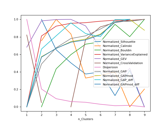
Optimal Number of Clusters
Find the optimal number of clusters based on different indices of quality of fit.
- Parameters:
data (np.ndarray) – An array (channels, times) of M/EEG data.
method (str) – The clustering algorithm to be passed into
nk.cluster().n_max (int) – Runs the clustering alogrithm from 1 to n_max desired clusters in
nk.cluster()with quality metrices produced for each cluster number.show (bool) – Plot indices normalized on the same scale.
**kwargs – Other arguments to be passed into
nk.cluster()andnk.cluster_quality().
- Returns:
DataFrame – The different quality scores for each number of clusters:
Score_Silhouette
Score_Calinski
Score_Bouldin
Score_VarianceExplained
Score_GAP
Score_GAPmod
Score_GAP_diff
Score_GAPmod_diff
See also
Examples
In [1]: import neurokit2 as nk

# Load the iris dataset
In [2]: data = nk.data("iris").drop("Species", axis=1)

# How many clusters
In [3]: results = nk.cluster_findnumber(data, method="kmeans", show=True)
cluster_quality()#
- cluster_quality(data, clustering, clusters=None, info=None, n_random=10, random_state=None, **kwargs)[source]#
Assess Clustering Quality
Compute quality of the clustering using several metrics.
- Parameters:
data (np.ndarray) – A matrix array of data (e.g., channels, sample points of M/EEG data)
clustering (DataFrame) – Information about the distance of samples from their respective clusters, generated from
cluster().clusters (np.ndarray) – Coordinates of cluster centers, which has a shape of n_clusters x n_features, generated from
cluster().info (dict) – Information about the number of clusters, the function and model used for clustering, generated from
cluster().n_random (int) – The number of random initializations to cluster random data for calculating the GAP statistic.
random_state (None, int, numpy.random.RandomState or numpy.random.Generator) – Seed for the random number generator. See for
misc.check_random_statefor further information.**kwargs – Other argument to be passed on, for instance
GFPas'sd'in microstates.
- Returns:
individual (DataFrame) – Indices of cluster quality scores for each sample point.
general (DataFrame) – Indices of cluster quality scores for all clusters.
Examples
In [1]: import neurokit2 as nk

# Load the iris dataset
In [2]: data = nk.data("iris").drop("Species", axis=1)

# Cluster
In [3]: clustering, clusters, info = nk.cluster(data, method="kmeans", n_clusters=3)

# Compute indices of clustering quality
In [4]: individual, general = nk.cluster_quality(data, clustering, clusters, info)

In [5]: general
Out[5]:
   n_Clusters  Score_Silhouette  ...  Score_GAP_sk  Score_GAPmod_sk
0         3.0          0.551192  ...        0.2113       976.778329

[1 rows x 12 columns]
References
Tibshirani, R., Walther, G., & Hastie, T. (2001). Estimating the number of clusters in a data set via the gap statistic. Journal of the Royal Statistical Society: Series B (Statistical Methodology), 63(2), 411-423.
Mohajer, M., Englmeier, K. H., & Schmid, V. J. (2011). A comparison of Gap statistic definitions with and without logarithm function. arXiv preprint arXiv:1103.4767.
Indices of fit#
fit_error()#
- fit_error(y, y_predicted, n_parameters=2)[source]#
Calculate the fit error for a model
Also specific and direct access functions can be used, such as
fit_mse(),fit_rmse()andfit_r2().- Parameters:
y (Union[list, np.array, pd.Series]) – The response variable (the y axis).
y_predicted (Union[list, np.array, pd.Series]) – The fitted data generated by a model.
n_parameters (int) – Number of model parameters (for the degrees of freedom used in R2).
- Returns:
dict – A dictionary containing different indices of fit error.
See also
fit_mse,fit_rmse,fit_r2Examples
In [1]: import neurokit2 as nk

In [2]: y = np.array([-1.0, -0.5, 0, 0.5, 1])

In [3]: y_predicted = np.array([0.0, 0, 0, 0, 0])

# Master function
In [4]: x = nk.fit_error(y, y_predicted)

In [5]: x
Out[5]:
{'SSE': np.float64(2.5),
 'MSE': np.float64(0.5),
 'RMSE': np.float64(0.7071067811865476),
 'R2': np.float64(0.7071067811865475),
 'R2_adjusted': np.float64(0.057190958417936755)}

# Direct access
In [6]: nk.fit_mse(y, y_predicted)
Out[6]: np.float64(0.5)

In [7]: nk.fit_rmse(y, y_predicted)
Out[7]: np.float64(0.7071067811865476)

In [8]: nk.fit_r2(y, y_predicted, adjusted=False)
Out[8]: np.float64(0.7071067811865475)

In [9]: nk.fit_r2(y, y_predicted, adjusted=True, n_parameters=2)
Out[9]: np.float64(0.057190958417936755)
fit_loess()#
- fit_loess(y, X=None, alpha=0.75, order=2)[source]#
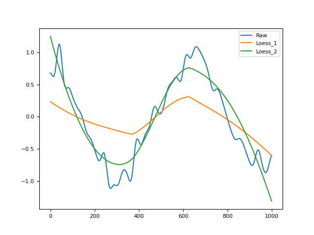
Local Polynomial Regression (LOESS)
Performs a LOWESS (LOcally WEighted Scatter-plot Smoother) regression.
- Parameters:
y (Union[list, np.array, pd.Series]) – The response variable (the y axis).
X (Union[list, np.array, pd.Series]) – Explanatory variable (the x axis). If
None, will treat y as a continuous signal (useful for smoothing).alpha (float) – The parameter which controls the degree of smoothing, which corresponds to the proportion of the samples to include in local regression.
order (int) – Degree of the polynomial to fit. Can be 1 or 2 (default).
- Returns:
array – Prediction of the LOESS algorithm.
dict – Dictionary containing additional information such as the parameters (
orderandalpha).
See also
Examples
In [1]: import pandas as pd

In [2]: import neurokit2 as nk

# Simulate Signal
In [3]: signal = np.cos(np.linspace(start=0, stop=10, num=1000))

# Add noise to signal
In [4]: distorted = nk.signal_distort(signal,
   ...:                               noise_amplitude=[0.3, 0.2, 0.1],
   ...:                               noise_frequency=[5, 10, 50])
   ...:

# Smooth signal using local regression
In [5]: pd.DataFrame({ "Raw": distorted, "Loess_1": nk.fit_loess(distorted, order=1)[0],
   ...:                "Loess_2": nk.fit_loess(distorted, order=2)[0]}).plot()
   ...:
Out[5]: <Axes: >
References
fit_mixture()#
- fit_mixture(X=None, n_clusters=2)[source]#
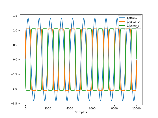
Gaussian Mixture Model
Performs a polynomial regression of given order.
- Parameters:
X (Union[list, np.array, pd.Series]) – The values to classify.
n_clusters (int) – Number of components to look for.
- Returns:
pd.DataFrame – DataFrame containing the probability of belonging to each cluster.
dict – Dictionary containing additional information such as the parameters (
n_clusters()).
See also
Examples
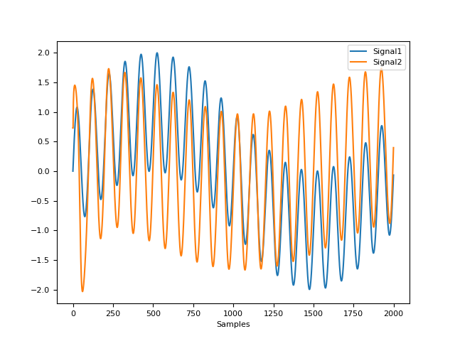
In [1]: import pandas as pd

In [2]: import neurokit2 as nk

In [3]: x = nk.signal_simulate()

In [4]: probs, info = nk.fit_mixture(x, n_clusters=2)  # Rmb to merge with main to return ``info``

In [5]: fig = nk.signal_plot([x, probs["Cluster_0"], probs["Cluster_1"]], standardize=True)
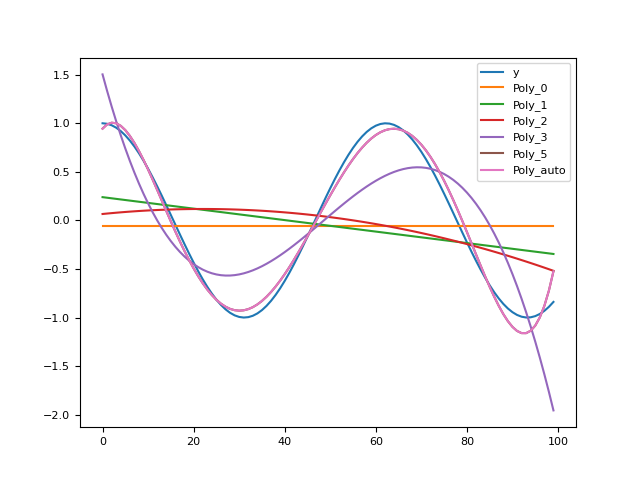
fit_polynomial()#
- fit_polynomial(y, X=None, order=2, method='raw')[source]#
Polynomial Regression
Performs a polynomial regression of given order.
- Parameters:
y (Union[list, np.array, pd.Series]) – The response variable (the y axis).
X (Union[list, np.array, pd.Series]) – Explanatory variable (the x axis). If
None, will treat y as a continuous signal.order (int) – The order of the polynomial. 0, 1 or > 1 for a baseline, linear or polynomial fit, respectively. Can also be
"auto", in which case it will attempt to find the optimal order to minimize the RMSE.method (str) – If
"raw"(default), compute standard polynomial coefficients. If"orthogonal", compute orthogonal polynomials (and is equivalent to R’spolydefault behavior).
- Returns:
array – Prediction of the regression.
dict – Dictionary containing additional information such as the parameters (
order) used and the coefficients (coefs).
See also
signal_detrend,fit_error,fit_polynomial_findorderExamples
In [1]: import pandas as pd

In [2]: import neurokit2 as nk

In [3]: y = np.cos(np.linspace(start=0, stop=10, num=100))

In [4]: pd.DataFrame({"y": y,
   ...:               "Poly_0": nk.fit_polynomial(y, order=0)[0],
   ...:               "Poly_1": nk.fit_polynomial(y, order=1)[0],
   ...:               "Poly_2": nk.fit_polynomial(y, order=2)[0],
   ...:               "Poly_3": nk.fit_polynomial(y, order=3)[0],
   ...:               "Poly_5": nk.fit_polynomial(y, order=5)[0],
   ...:               "Poly_auto": nk.fit_polynomial(y, order='auto')[0]}).plot()
   ...:
Out[4]: <Axes: >
Any function appearing below this point is not explicitly part of the documentation and should be added. Please open an issue if there is one.
Submodule for NeuroKit.
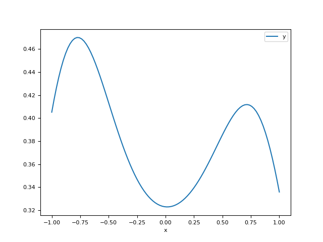
- density_bandwidth(x, method='KernSmooth', resolution=401)[source]#
Bandwidth Selection for Density Estimation
Bandwidth selector for
density()estimation. Seebw_methodargument inscipy.stats.gaussian_kde().The
"KernSmooth"method is adapted from thedpik()function from the KernSmooth R package. In this case, it estimates the optimal AMISE bandwidth using the direct plug-in method with 2 levels for the Parzen-Rosenblatt estimator with Gaussian kernel.- Parameters:
x (Union[list, np.array, pd.Series]) – A vector of values.
method (float) – The bandwidth of the kernel. The larger the values, the smoother the estimation. Can be a number, or
"scott"or"silverman"(seebw_methodargument inscipy.stats.gaussian_kde()), or"KernSmooth".resolution (int) – Only when
method="KernSmooth". The number of equally-spaced points over which binning is performed to obtain kernel functional approximation (seegridsizeargument inKernSmooth::dpik()).
- Returns:
float – Bandwidth value.
See also
densityExamples
In [1]: import neurokit2 as nk

In [2]: x = np.random.normal(0, 1, size=100)

In [3]: bw = nk.density_bandwidth(x)

In [4]: bw
Out[4]: np.float64(0.4470044832800954)

In [5]: nk.density_bandwidth(x, method="scott")
Out[5]: np.float64(0.3981071705534972)

In [6]: nk.density_bandwidth(x, method=1)
Out[6]: 1

In [7]: x, y = nk.density(signal, bandwidth=bw, show=True)
References
Jones, W. M. (1995). Kernel Smoothing, Chapman & Hall.
- fit_polynomial_findorder(y, X=None, max_order=6)[source]#
Polynomial Regression.
Find the optimal order for polynomial fitting. Currently, the only method implemented is RMSE minimization.
- Parameters:
y (Union[list, np.array, pd.Series]) – The response variable (the y axis).
X (Union[list, np.array, pd.Series]) – Explanatory variable (the x axis). If ‘None’, will treat y as a continuous signal.
max_order (int) – The maximum order to test.
- Returns:
int – Optimal order.
See also
fit_polynomialExamples
import neurokit2 as nk
y = np.cos(np.linspace(start=0, stop=10, num=100))
nk.fit_polynomial_findorder(y, max_order=10)
9